Evolution of diversity in metabolic strategies
- Departamento de Física, Universidade Federal do Paraná, Brazil
- Department of Physics, University of Santiago of Chile (USACH), Chile
- Department of Mathematics and Department of Zoology, University of British Columbia, Canada
Figures
Figure 1
Snapshots illustrating the beginning, intermediate, and advanced stages of evolution under a linear constraint, .
A video of the entire evolutionary process can be found here, frames are recorded every 200 time units until t=30,000 and then, to better illustrate slow neutral evolution, the frame recording times ti were defined as a geometric progression . Other parameter values were , for , and .
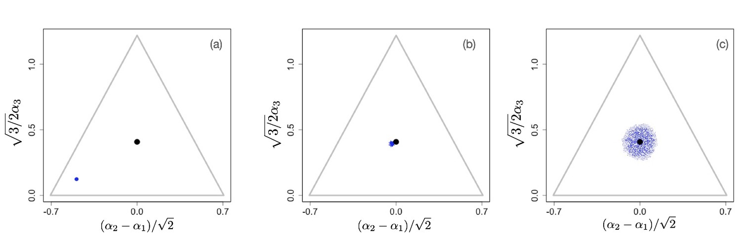
Figure 2
Example of evolutionary dynamics for , showing convergence to the singular point given by Equation 4 (and indicated by the black dot), but no subsequent diversification.
The corresponding video can be found here , each frame in the video is separated by 1,000 time steps. Other parameter values were , for , and .
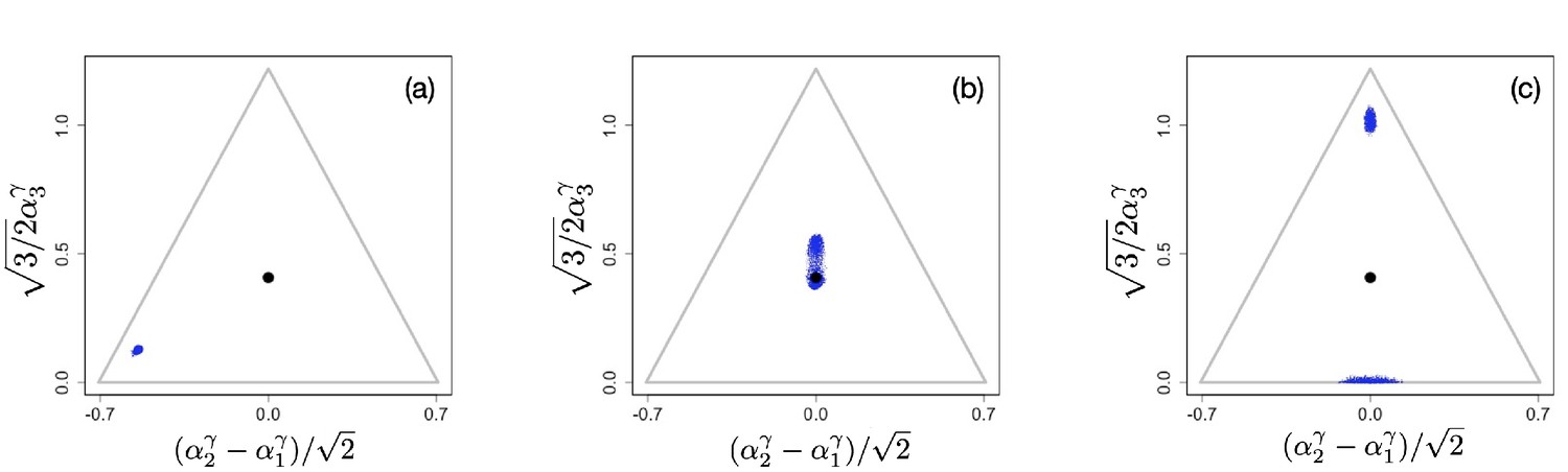
Figure 3
Example of evolutionary dynamics for , showing initial convergence to the singular point (indicated by the black dot) and subsequent diversification into three specialists, each consuming exclusively one of the three resources.
The corresponding video can be found here, each frame in the video is separated by 1,000 time steps. Other parameter values were , for , and .
Appendix 1—figure 1
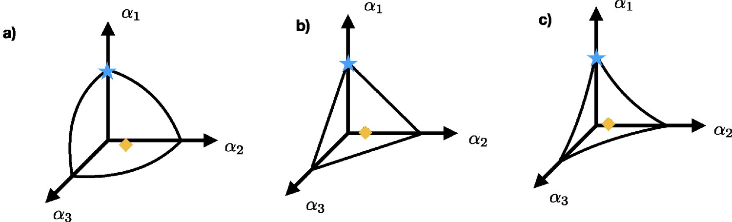
Three possible surfaces defined by a tradeoff: (a) shows the concave surface for the case , while (b) and (c) show the surface for the cases and , respectively.
The blue star and the orange diamond represent possible strategies. Individuals with strategy represented by the blue star obtain their nutrients only from resource s1 while the individuals that adopt strategy indicated by the orange diamond uptake nutrients from all three resources.
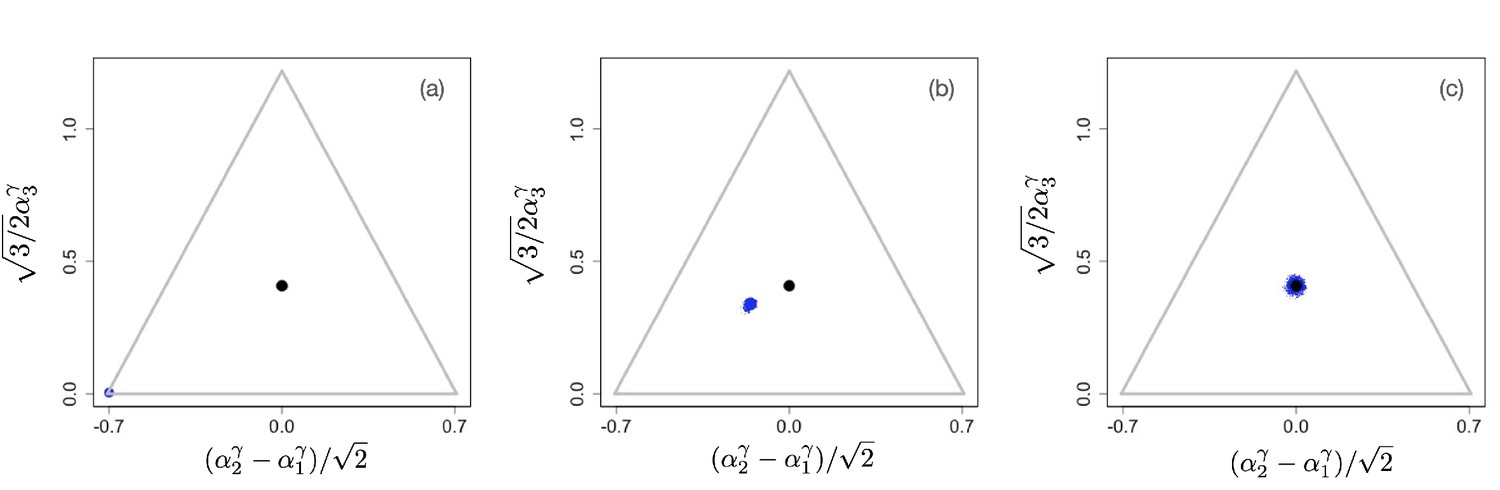
Appendix 1—figure 2
Example of evolutionary dynamics for and , showing convergence to the singular point and subsequent diversification only in the direction.
(Note that the dynamics are shown in the original α-phenotype space.) The corresponding video can be found here, each frame in the video is separated by 2,000 time steps. Other parameter values were , for , and .
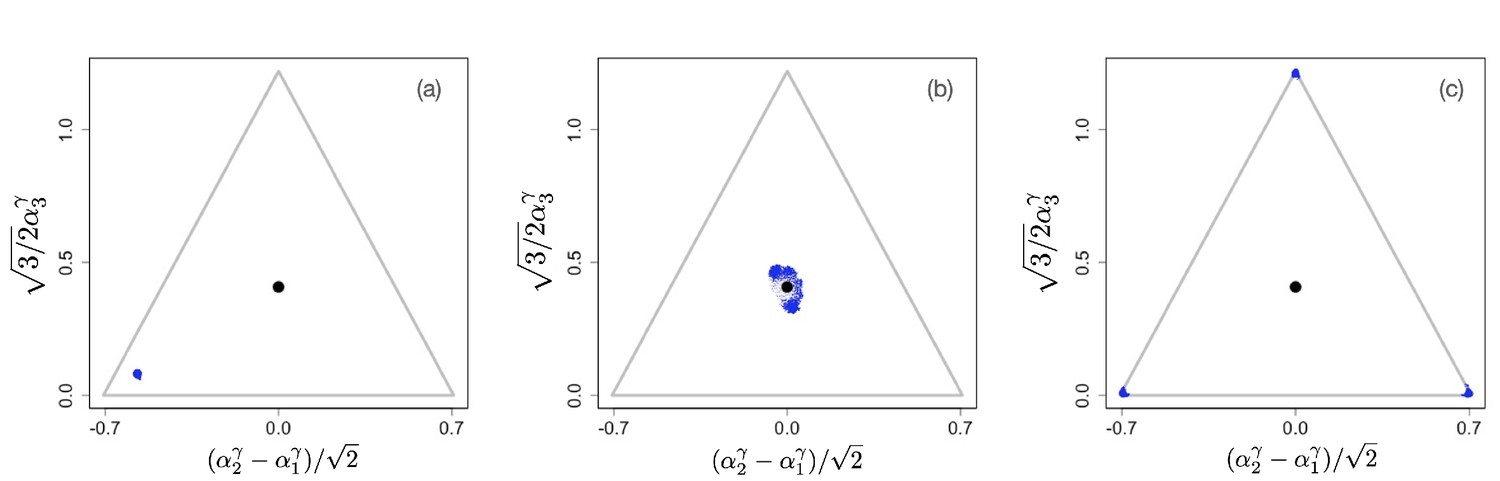
Appendix 1—figure 3

Example of evolutionary dynamics for and , showing convergence to the singular point and subsequent diversification only in directions.
(Note that the dynamics are shown in the original α-phenotype space.) The corresponding video can be found here, each frame in the video is separated by 2000 time steps. Other parameter values were , for , and .
Appendix 1—figure 4
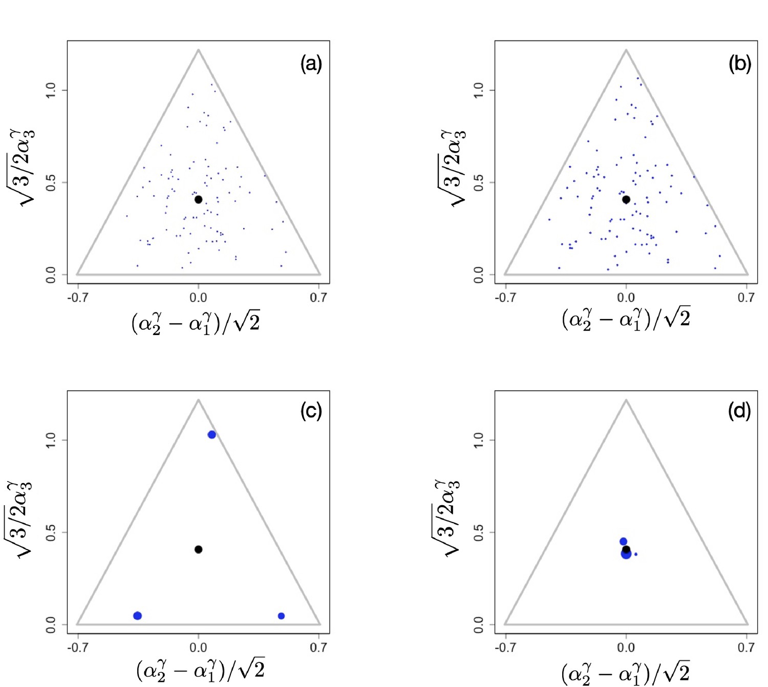
Initial population configuration of 100 randomly placed clusters in the phenotypic simplex (a), final configurations after 5,000,000 time units for (b), (c), and (d). Videos of the entire ecological processes can be found here, time interval between frames increased as a geometric progression, . Other parameter values were , for , and .
Author response image 1
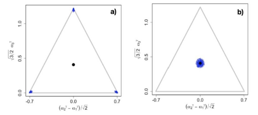
Snapshots illustrating the end of the evolutionary dynamics for (a) = 0.
99 and (b) = 1.01. The video of the entire evolutionary process can be found at https://figshare.com/s/f65ed0bf9b4305e9018f .
Additional files
Download links
A two-part list of links to download the article, or parts of the article, in various formats.
Downloads (link to download the article as PDF)
Open citations (links to open the citations from this article in various online reference manager services)
Cite this article (links to download the citations from this article in formats compatible with various reference manager tools)
Evolution of diversity in metabolic strategies
eLife 10:e67764.
https://doi.org/10.7554/eLife.67764


