An oscillating computational model can track pseudo-rhythmic speech by using linguistic predictions
- Language and Computation in Neural Systems group, Max Planck Institute for Psycholinguistics, Netherlands
- Donders Centre for Cognitive Neuroimaging, Radboud University, Netherlands
- Department of Cognitive Neuroscience, Faculty of Psychology and Neuroscience, Maastricht University, Netherlands
Figures
Figure 1

Proposed interaction between speech timing and internal linguistic models.
(A) Isochronous production and expectation when there is a weak internal model (even distribution of node activation). All speech units arrive around the most excitable phase. (B) When the internal model of the producer does not align with the model of the receiver temporal alignment and optimal communication fails. (C) When both producer and receiver have a strong internal model, speech is non-isochronous and not aligned to the most excitable phase, but fully expected by the brain. (D) Expected time is a constraint distribution in which the center can be shifted due to linguistic constraints.
Figure 2 with 3 supplements

Word frequency modulates word duration.
(A) Example of mono- and bi-syllabic words of different word frequencies in brackets (van=from, zijn=be, snel=fast, stem=voice, hebben=have, eten=eating, volgend=next, toekomst=future). Text in the graph indicates the mean word duration. (B) Relationship between word frequency and duration. Darker colors mean more values. (C) same as (B) but separately for mono- and bi-syllabic words. (D) Relationship character amount and word duration. The longer the words, the longer the duration (left). The increase in word duration does not follow a fixed number per character as duration as measured by rate increases. (E) same as (D) but for number of syllables. Red dots indicate the mean.
Figure 2—figure supplement 1
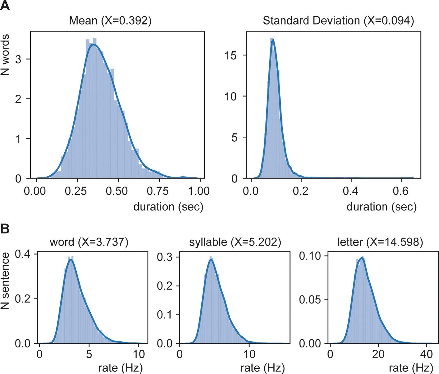
Distribution of mean duration (A) and of average rate (B).
Figure 2—figure supplement 2
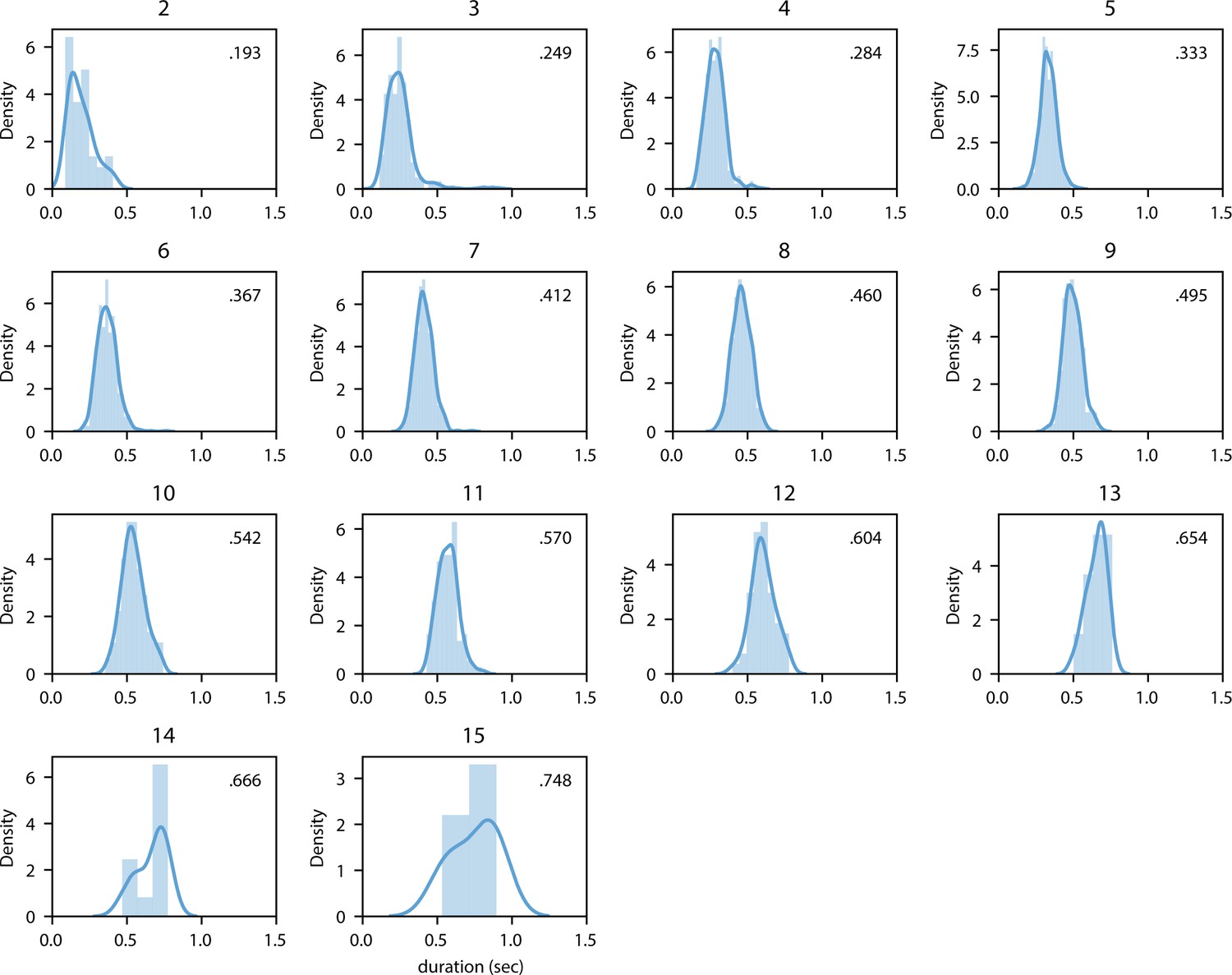
Distribution of mean duration split up for word length (in characters).
Figure 2—figure supplement 3
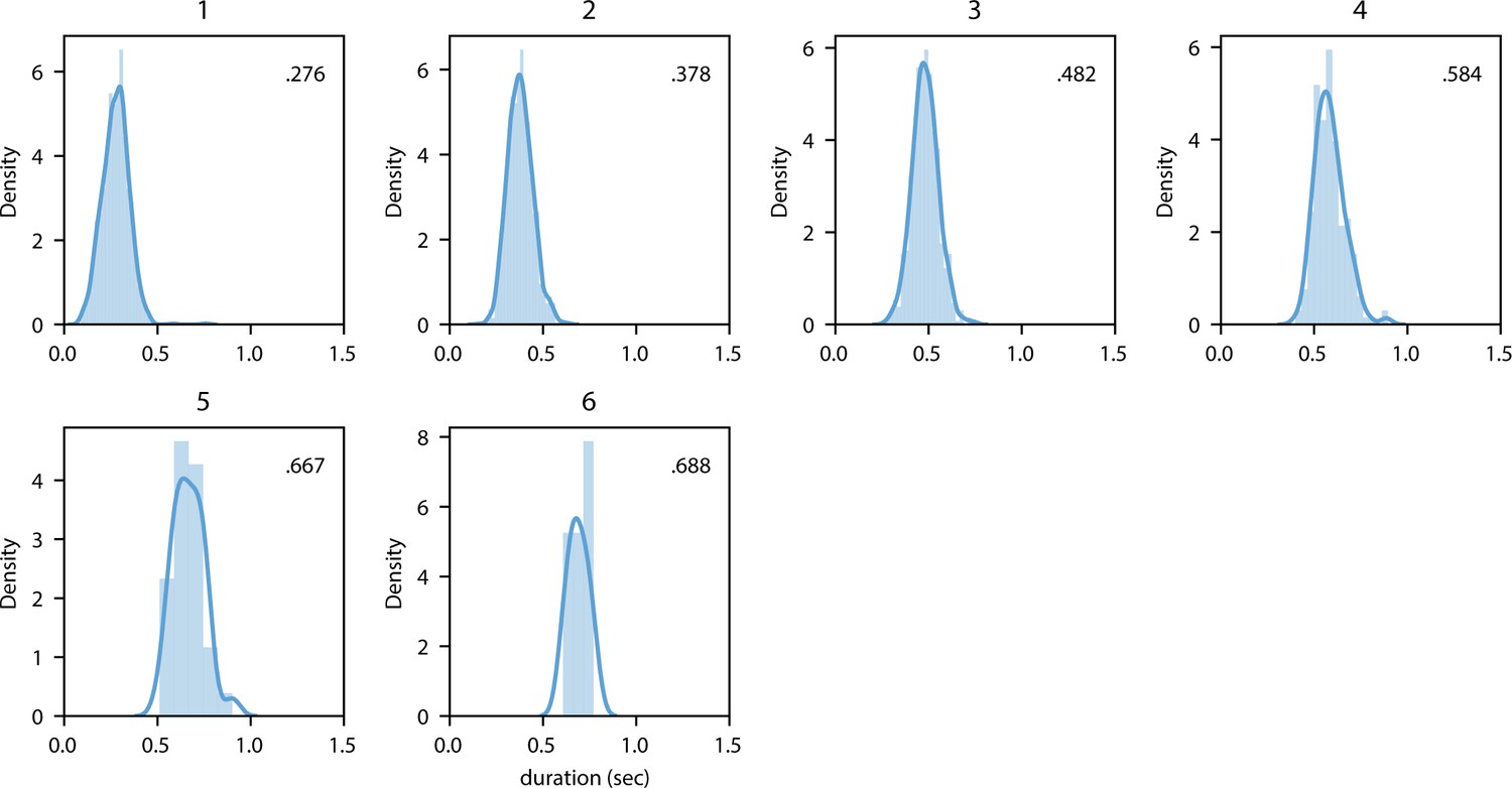
Distribution of mean duration split up for syllable length.
Figure 3 with 2 supplements
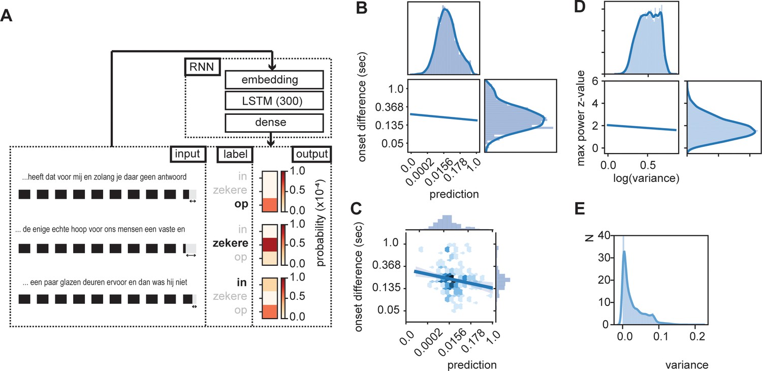
RNN output influence word onset differences.
(A) Sequences of 10 words were entered in an RNN in order to predict the content of the next word. Three examples are provided of input data with the label (bold word) and probability output for three different words. The regression model showed a relation between the duration of last word in the sequence and the predictability of the next word such that words were systematically shorter when the next word was more predictable according to the RNN output (illustrated here with the shorted black boxes). (B) Regression line estimated at mean value of word duration and bigram. (C) Scatterplot of prediction and onset difference of data within ± 0.5 standard deviation of word duration and bigram. Note that for (B) and (C), the axes are linear on the transformed values. (D) Regression line for the correlation between logarithm of variance of the prediction and theta power. (E) None-transformed distribution of variance of the predictions (within a sentence). Translation of the sentences in (A) from top to bottom: ‘... that it has for me and while you have no answer [on]’, ‘... the only real hope for us humans is a firm and [sure]’, ‘... a couple of glass doors in front and then it would not have been [in]’.
Figure 3—figure supplement 1
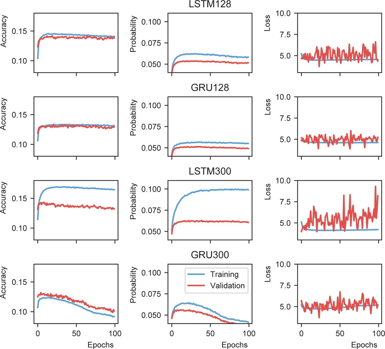
Recurrent neural network evaluation.
Probability is defined as the mean of the model output value at the node representing the next word.
Figure 3—figure supplement 2
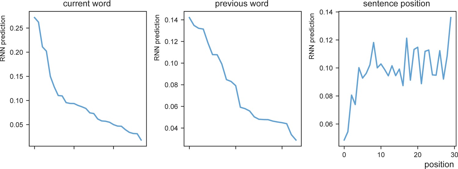
RNN prediction distributions.
RNN prediction dependent on the current word (left), previous word (middle), or sentence position (right). Words with generally high average RNN prediction were for current words ‘je’,’te’,’ik’,’de’,’van’ (‘you’,’to’,’I’,’the’,’from’) and previous words ‘dan’,’met’,’ook’,’voor’,’op’ (‘than’,’with’,’also’,’for’,’on’). The later the position the stronger the RNN prediction on average.
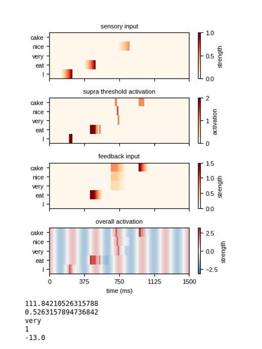
Figure 4
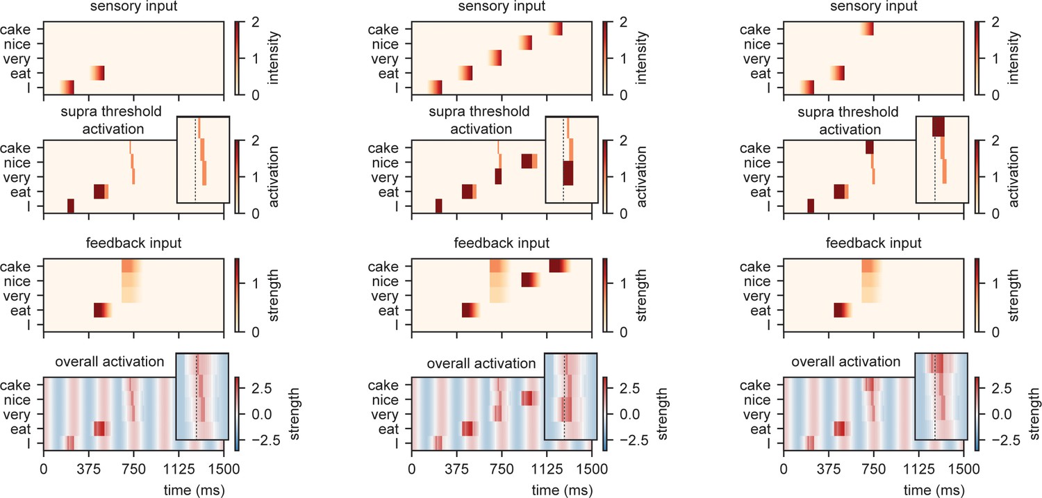
Model output for different sentences.
For the supra-threshold activation dark red indicates activation which included input from l+1 as well as l1, orange indicates activation due to l+1 input. Feedback at different strengths causes phase dependent activation (left). Suprathreshold activation is reached earlier when a highly predicted stimulus (right) arrives, compared to a mid-level predicted stimulus (middle).
Figure 5
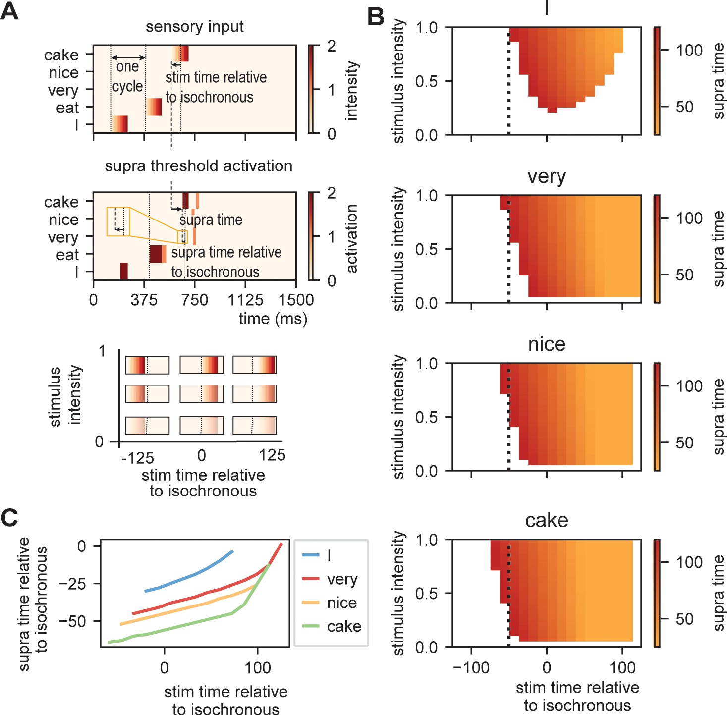
Model output on processing efficiency.
(A) Input given to the model. Sensory input is varied in intensity and timing. We extract the time of activation relative to stimulus onset (supra-time) and relative to isochrony onset. (B) Time of presentation influences efficiency. Outcome variable is the time at which the node reached threshold activation (supra-time). The dashed line is presented to ease comparison between the four content types. White indicates that threshold is never reached. (C) Same as (B), but estimated at a threshold of 0.53 showing that oscillations regulate feedforward timing. Panel (C) shows that the earlier the stimuli are presented (on a weaker point of the ongoing oscillation), the longer it takes until supra-threshold activation is reached. This figure shows that timing relative to the ongoing oscillation is regulated such that the stimulus activation timing is closer to isochronous. Line discontinuities are a consequence of stimuli never reaching threshold for a specific node.
Figure 6 with 2 supplements

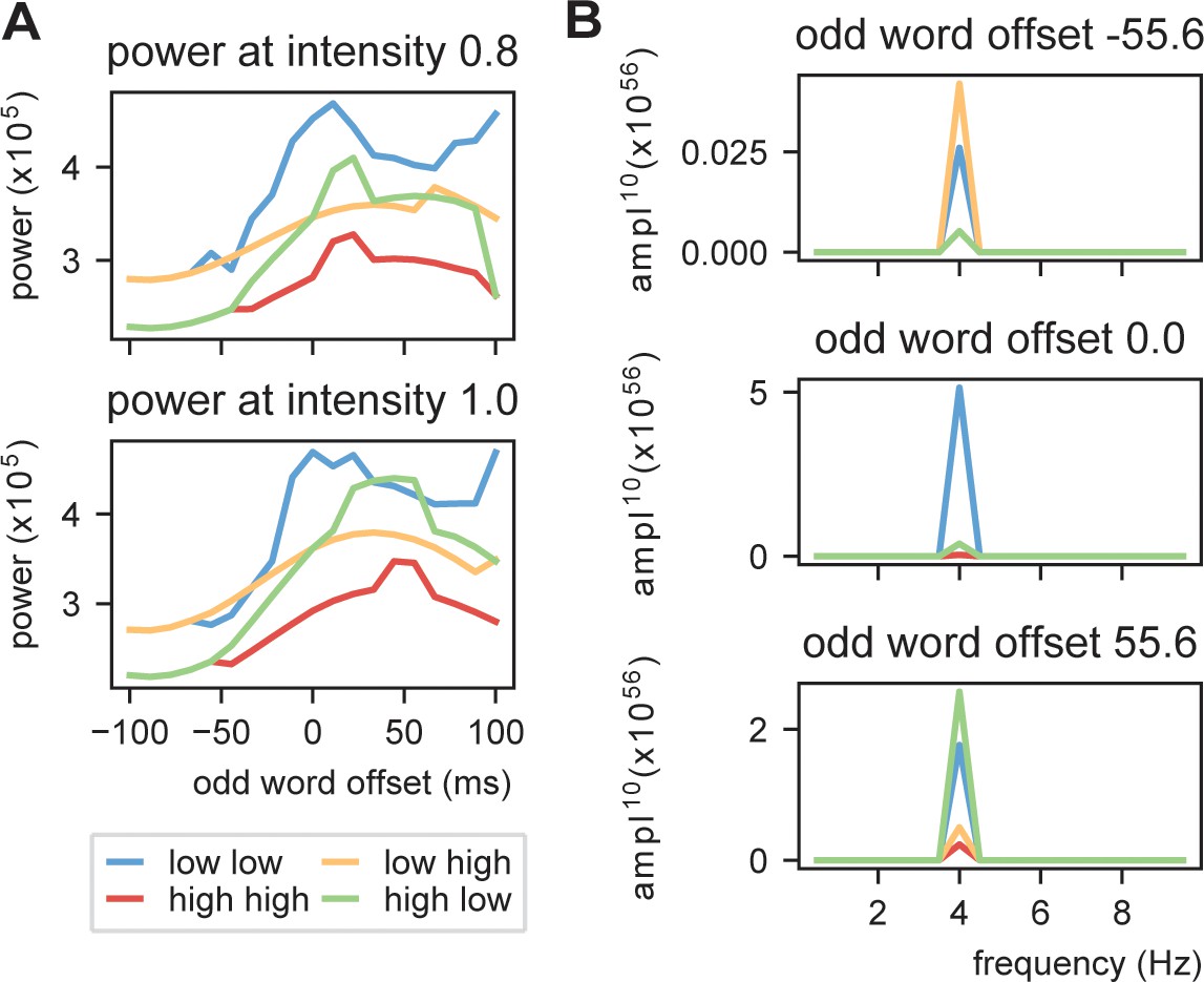
Model output on rhythmicity.
(A) We presented the model with repeating (A, B) stimuli with varying internal models. We extracted the power spectra and peak activity at various odd stimulus offsets and stimulus intensities. (B) Strength of 4 Hz power depends on predictability in the stream. When predictability is alternated between low and high, activation is more rhythmic when the predictable odd stimulus arrives earlier and vice versa. (C) Power across different internal models at intensity of 0.8 and 1.0 (different visualization than B). (D) Magnitude spectra at three different odd word offsets at 1.0 intensity. To more clearly illustrate the differences, the magnitude to the power of 20 is plotted.
Figure 6—figure supplement 1
Power at 4 Hz using linearly increasing sensory input.
Conventions of panel A, B are the same as in Figure 6C,D, respectively.
Figure 6—figure supplement 2
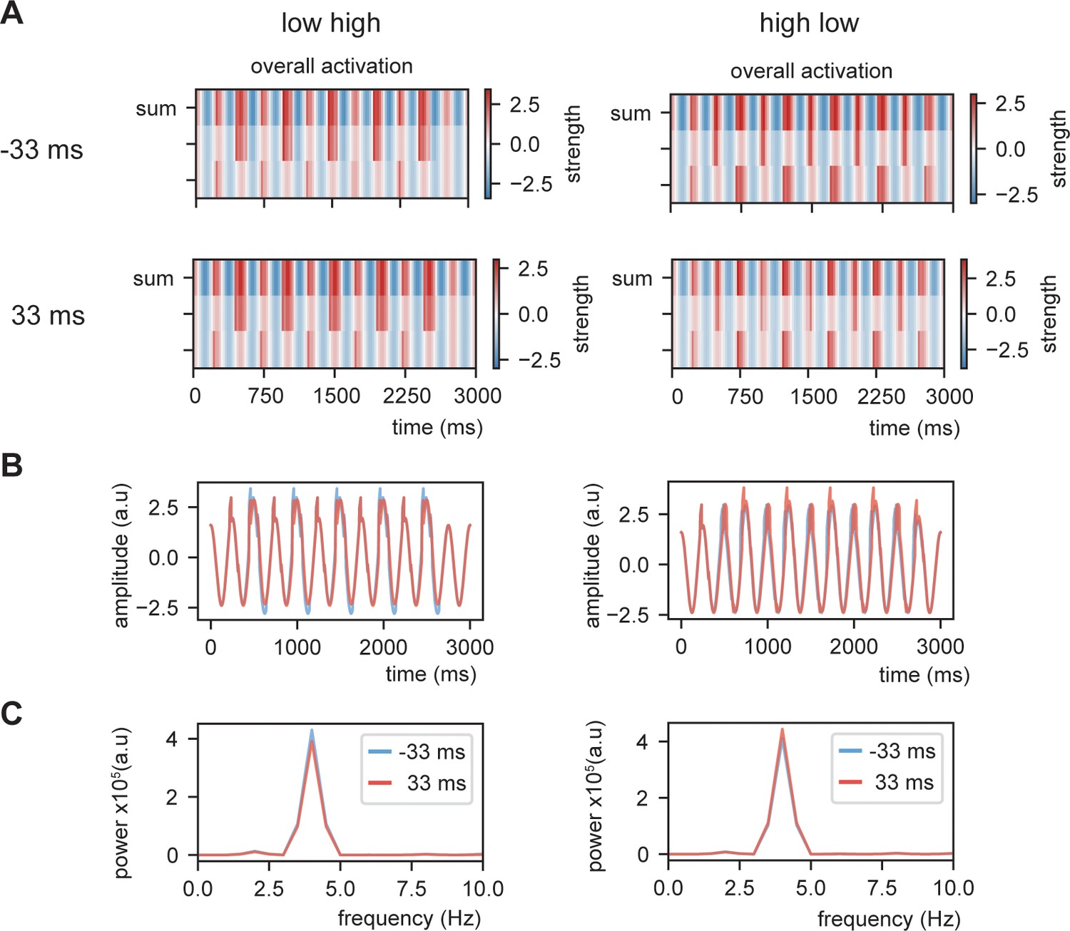
Example of overall activation at threshold 0.8 (Gaussian shaped input).
(A) Overall activation for individual nodes and summed activation. (B) Overall summed activation as time course. (C) Power spectra of the different delays and conditions. Dependent on the internal language model, the power is stronger at the -33 ms or 33 ms delay condition.
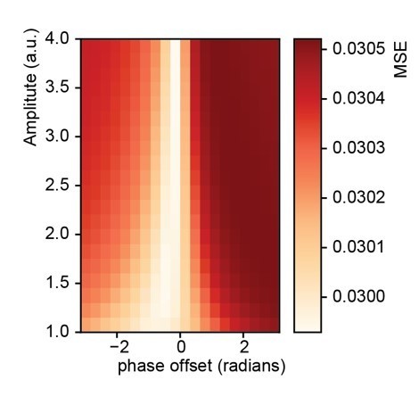
Figure 7

Fit between real and expected time shift dependent on predictability.
(A) Phase offset and amplitude of the oscillation modulate the fit to the word-to-word onset durations. (B) Histogram of the predictions created by the deep neural net. (C) Histogram of the relative time shift transformation at phase of −0.15π and amplitude of 1.5.
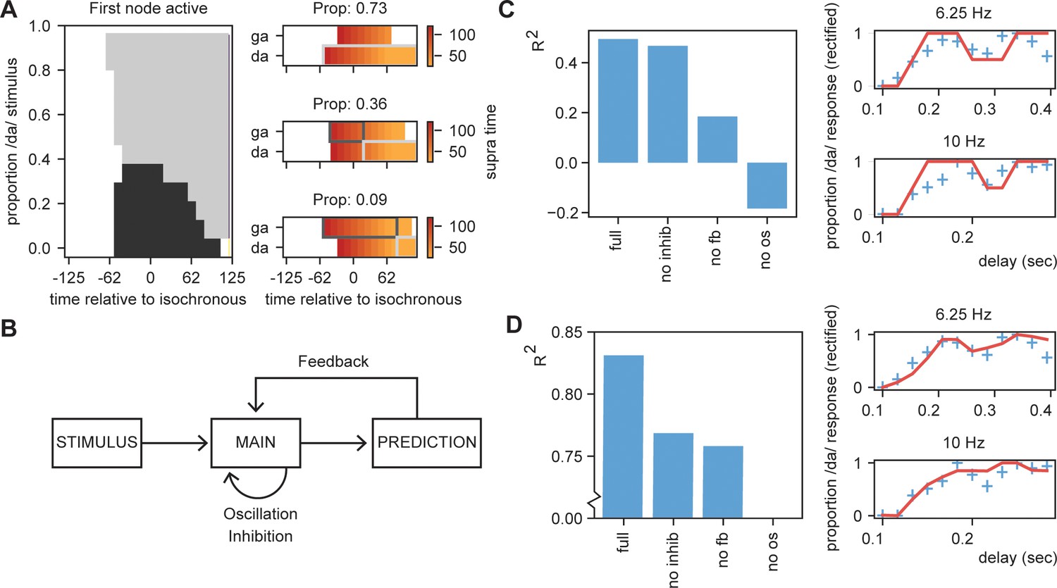
Figure 8 with 1 supplement
Results for /daga/ illusions.
(A) Modulations due to ambiguous input at different times. Illustration of the node that is active first. Different proportions of the /da/ stimulus show activation timing modulations at different delays. (B) Summary of the model and the parameters altered for the empirical fits in (C) and (D). (C). R2 for the grid search fit of the full model using the first active node as outcome variable, a model without inhibition (no inhib), without uneven feedback (no fb), or without an oscillation (no os). The right panel shows the fit of the full model on the rectified behavioral data of Ten Oever and Sack, 2015. Blue crossed indicate rectified data and red lines indicate the fit. (D) is the same as (C) but using the average activity instead of the first active node. Removing the oscillation results in an R2 less than 0.
Figure 8—figure supplement 1
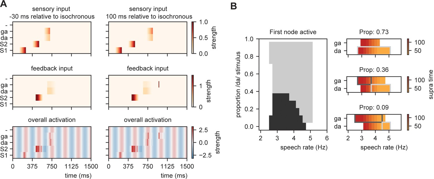
Explaining speech timing illusions.
(A) Model activation of two example delays for the fitting (Figure 8A). (B) Modulations due to ambiguous input at different speech rates. Illustration of the node that is active first. Different proportions of the /da/ stimulus show activation timing modulations at different speech rates. Conventions are the same as Figure 8.
Figure 9
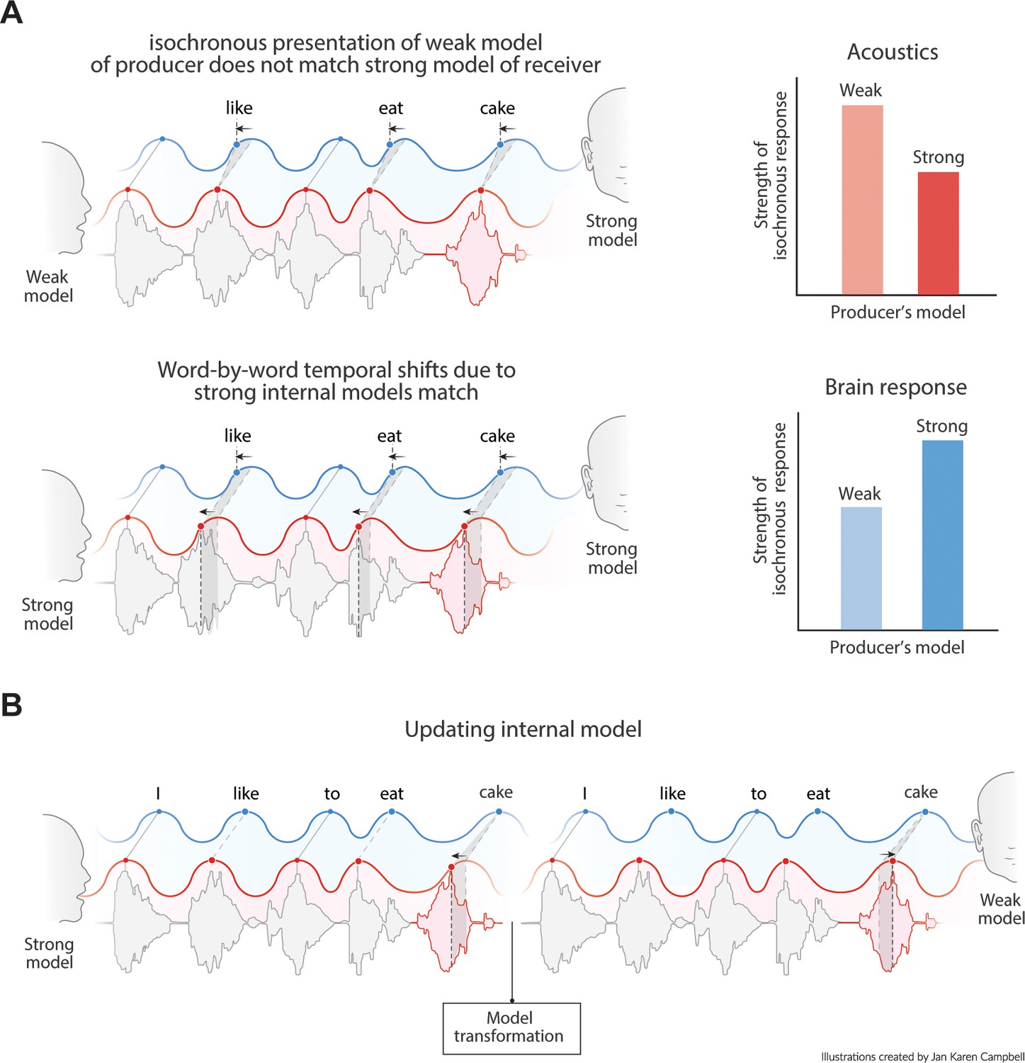
Predictions of the model.
(A) Acoustics signals will be more isochronous when a producer has a weak versus a strong internal model (top right). When the producer’s strong model matches the receiver’s model, the brain response will be more isochronous for less isochronous acoustic input. (B) When a producer realizes the model of the receiver is weak, it might transform its model and thereby their speech timing to match the receiver’s expectations.
Author response image 1
Author response image 2
Tables
Table 1
Summary of regression model for logarithm of onset difference of words.
| Variable | Trans | B | β | SE | t | p | VIF |
|---|---|---|---|---|---|---|---|
| Intercept | x | 0.9719 | 0.049 | 19.764 | <0.001 | ||
| RNN prediction | x (1/6) | −0.3370 | −0.0862 | 0.047 | −7.163 | <0.001 | 1.5 |
| Bigram | log(x) | −0.0118 | −0.0316 | 0.005 | −2.424 | 0.015 | 1.8 |
| Word frequency W-1 | x | 0.0049 | 0.0076 | 0.009 | 0.546 | 0.585 | 2.0 |
| Mean duration W-1 | log(x) | 1.1206 | 0.7003 | 0.022 | 50.326 | <0.001 | 2.0 |
| Syllable Rate | x | −0.1033 | −0.2245 | 0.004 | −23.014 | <0.001 | 1.0 |
-
Model R2 = 0.542. Trans = transformation, W-1 = previous word, B = unstandardized coefficient, β = standardized coefficient, SE = standard error, t = t value, p = p value, VIF = variance inflation factor.
Table 2
Example of a language model.
This model has seen three sentences at different probabilities. Rows represent the prediction for the next word, e.g., /I/ predicts /eat/ at a probability of 1, but after /eat/ there is a wider distribution.
| I | Eat | Very | Nice | Cake | |
|---|---|---|---|---|---|
| I | 0 | 1 | 0 | 0 | 0 |
| eat | 0 | 0 | 0.2 | 0.3 | 0.5 |
| very | 0 | 0 | 0 | 1 | 0 |
| nice | 0 | 0 | 0 | 0 | 1 |
| cake | 0 | 0 | 0 | 0 | 0 |
Table 3
Predictions from the current model.
| When there is a flat constraint distribution over an utterance (e.g., when probabilities are uniform over the utterance), the acoustics of speech should naturally be more isochronous (Figures 9A and 3D,E). |
| If speech timing matches the internal language model, brain responses should be more isochronous even if the acoustics are not (Figure 9A). |
| The more similar the internal language models of two speakers, the more effective they are in ‘entraining’ each other’s brain. |
| If speakers suspect their listener to have a flatter constraint distribution than themselves (e.g., the environment is noisy, or the speakers are in a second language context), they adjust to the distribution by speaking more isochronous (Figure 9B). |
| One adjusts the weight of the constraint distribution to a hierarchical level when needed. For example, when there is noise, participants adjust to the rhythm of primary auditory cortex instead of higher order language models. As a consequence, they speak more isochronous. |
| The theoretical account provides various predictions that are listed in this table. |
Additional files
-
Supplementary file 1
Summary of regression model for logarithm of word duration.
- https://cdn.elifesciences.org/articles/68066/elife-68066-supp1-v2.docx
-
Transparent reporting form
- https://cdn.elifesciences.org/articles/68066/elife-68066-transrepform-v2.pdf
Download links
A two-part list of links to download the article, or parts of the article, in various formats.
Downloads (link to download the article as PDF)
Open citations (links to open the citations from this article in various online reference manager services)
Cite this article (links to download the citations from this article in formats compatible with various reference manager tools)
An oscillating computational model can track pseudo-rhythmic speech by using linguistic predictions
eLife 10:e68066.
https://doi.org/10.7554/eLife.68066


