Coding of chromatic spatial contrast by macaque V1 neurons
- Graduate Program in Neuroscience, University of Washington, United States
- Department of Physiology and Biophysics, Washington National Primate Research Center, University of Washington, United States
Figures
Figure 1
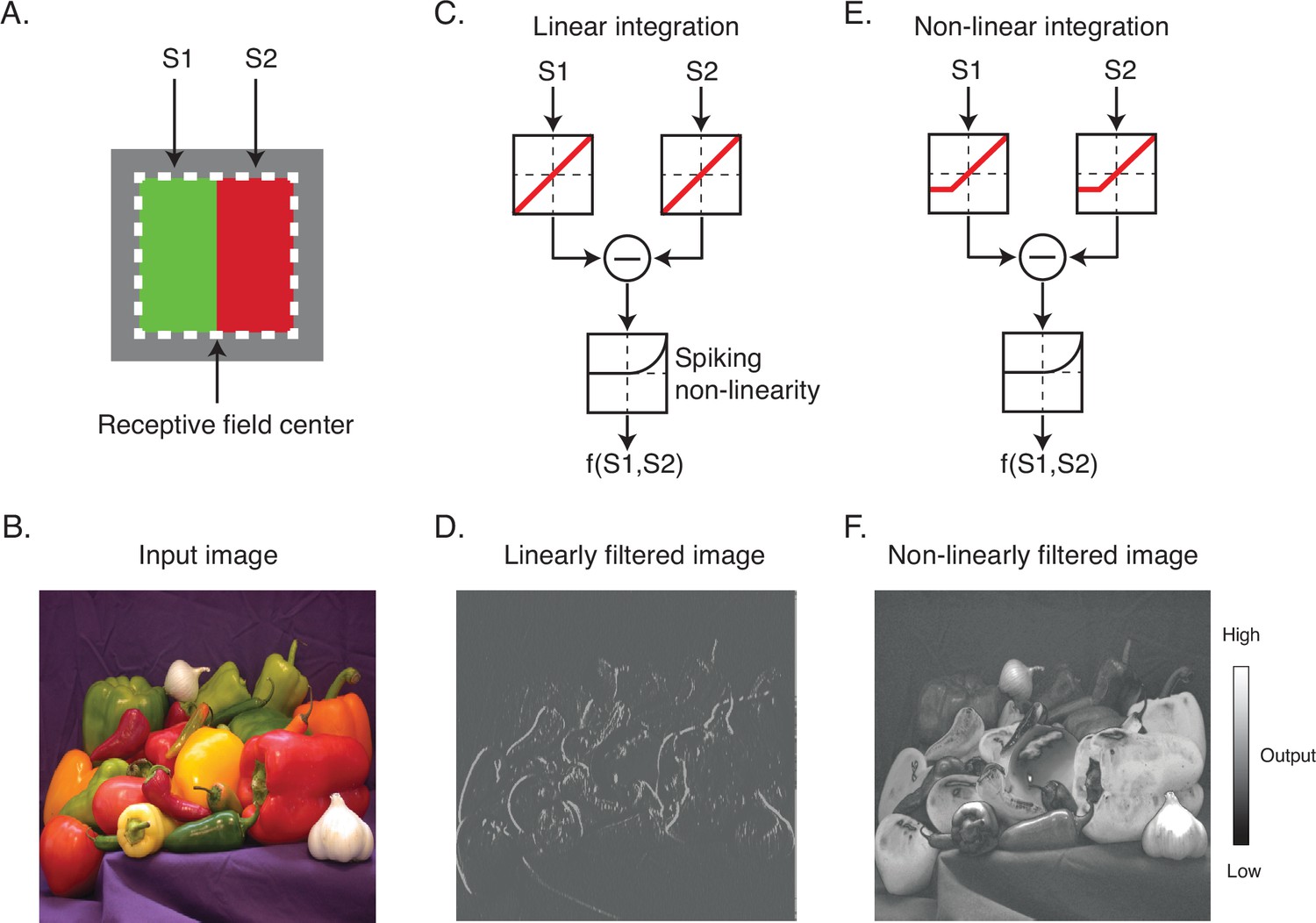
Linear and nonlinear image filtering.
(A) A hypothetical V1 DO cell that is excited by a red light on one side of its receptive field (RF) and a green light on the other. S1 and S2 represent stimulation of the two subfields of the RF. (B) An example natural image. (C) A linear spatial filter that sums the drive from each subfield and generates a response via a spiking nonlinearity. Note that the drive from each subfield is combined linearly before being transformed by the spiking nonlinearity. (D) Linearly filtered image using filter in (C). (E) A nonlinear spatial filter that partially rectifies S1 and S2 prior to summation. (F) Nonlinearly filtered image using filter in (E). DO, double-opponent.
Figure 2 with 5 supplements
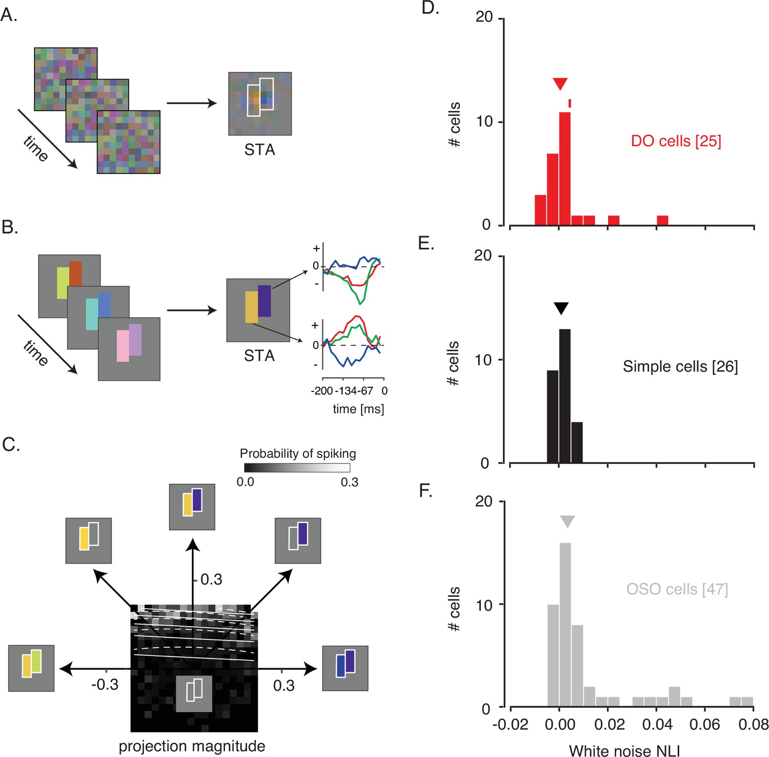
White noise analysis of RF structure and spatial integration.
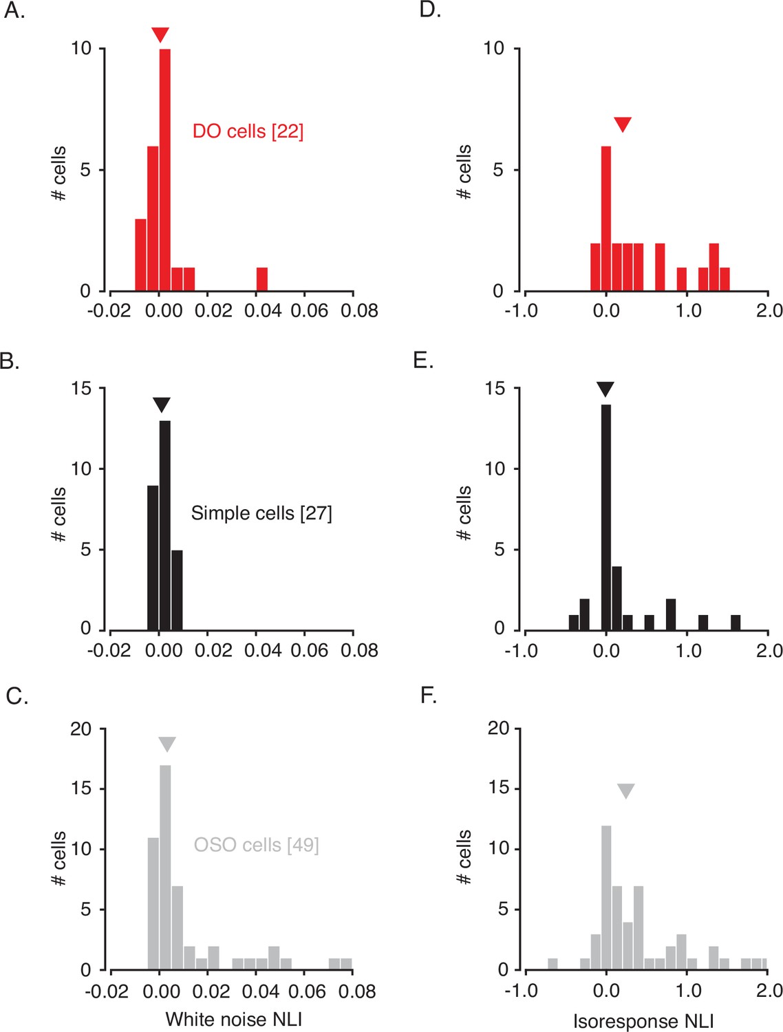
(A) Pixel white noise stimulus (left), spike-triggered average (STA; right). Two sets of contiguous pixels were yoked to create two hyperpixels, each of which stimulated one RF subfield (white outlines). (B) Hyperpixel white noise stimulus (left) and STA at the peak frame (middle). Red, green, and blue curves (right) represent the average red, green, and blue phosphor intensities, relative to background, as a function of time before a spike. (C) A firing rate map for the example DO cell. The probability of spiking (grayscale) is plotted as a function of projection magnitudes of the hyperpixel stimulus onto the right and left halves of the STA (the 45° and 135° directions, respectively). Solid and dashed white lines are contours of constant spiking probability from GLM and GQM fits to the data, respectively. The firing rate map is binned to facilitate visualization, but models were fit to unbinned data. (D) Histogram of white noise NLIs for DO cells. The NLI of the example neuron is marked with a tick, and the median is marked with a triangle. (E) Same as (D) but for simple cells. (F) Same as (D) but for the other spatially opponent cells. DO, double-opponent; GLM, generalized linear model; GQM, generalized quadratic model; NLI, nonlinearity index; RF, receptive field.
Figure 2—figure supplement 1

Comparison of the effective stimulus contrast across the three phases of the experiment.
(A) Stimuli from Phase 1 (black) and Phase 2 (red) were projected onto the spatial–temporal–chromatic STA shown in Figure 2B. Projection magnitudes of both stimuli occupy only a small region of the display gamut (dashed gray rectangle). (B) Two-dimensional histogram of the Phase 1 projections shown in (A, C). Same as (B) but for the Phase 2 stimuli. (D) The probability of spiking (the ratio of spike triggering to total stimuli) as a function of hyperpixel stimulus projections onto the two halves of the STA. Projection magnitudes are shown from the 5th to the 95th percentile. Within this range, the probability of a spike increases approximately as a linear combination of the stimulus projections, but this range is a small fraction of what can be achieved on the display. STA, spike-triggered average.
Figure 2—figure supplement 2

Comparison of firing rates across the three phases of the experiment.
(A) Scatterplot of the firing rates (mean ± sem) in response to pixel and hyperpixel white noise for DO cells (red), simple cells (black), and OSO cells (gray). (B) Same as (A) but comparing responses to Phase 3 stimuli and hyperpixel white noise. DO, double-opponent; OSO, other spatially opponent.
Figure 2—figure supplement 3
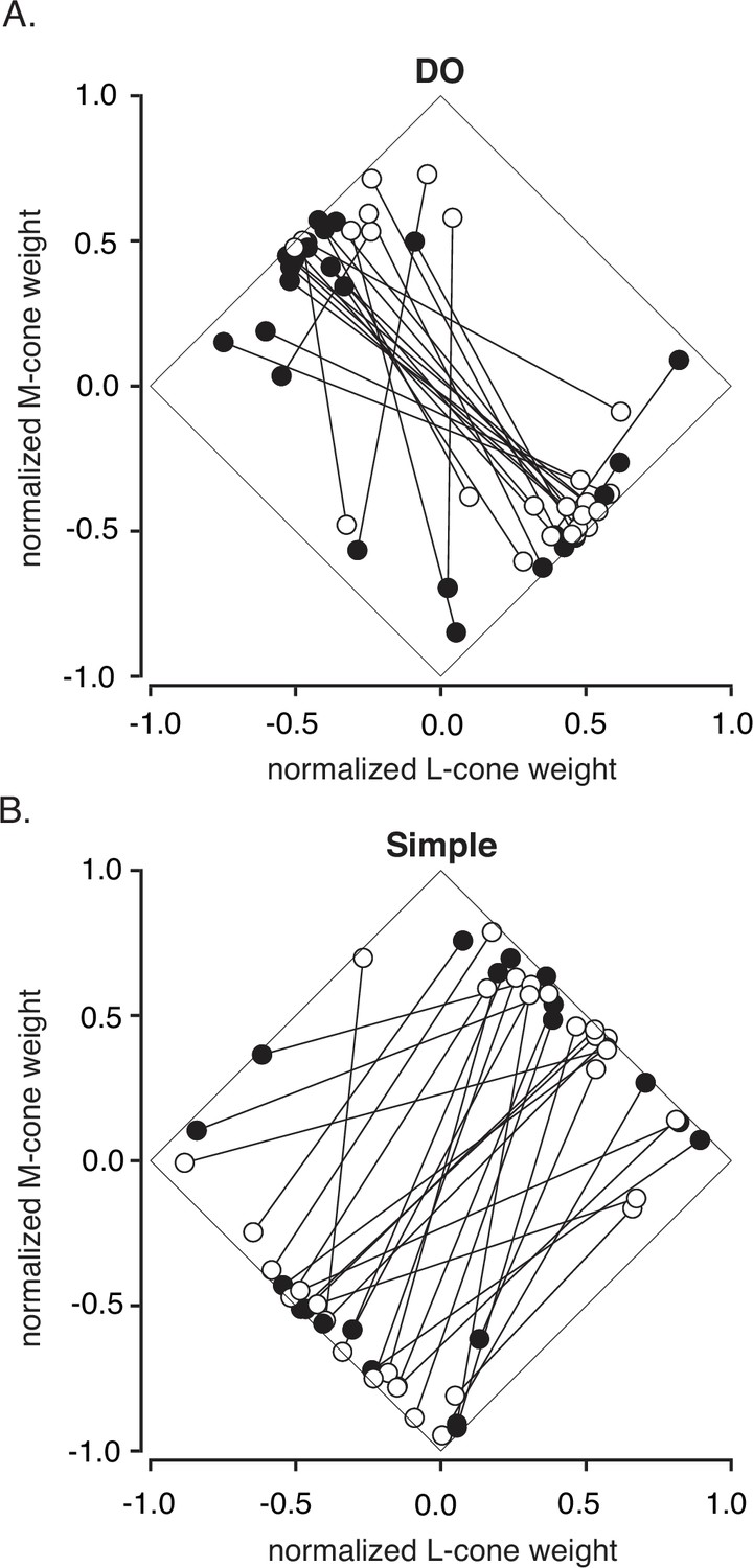
Cone weights for DO cells (A) and simple cells (B) derived from each hyperpixel STA.
Each neuron is represented by a line joining two circles. Circle position indicates normalized cone weights and fill indicates the sign of the S-cone weight (filled = positive, unfilled = negative). DO, double-opponent; STA, spike-triggered average.
Figure 2—figure supplement 4
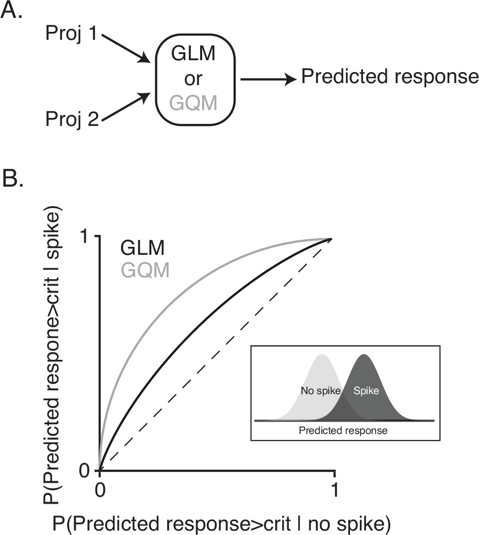
Overview of hyperpixel white noise nonlinearity index calculation.
(A) Probability of spiking was predicted as a function of projection magnitudes onto the two halves of the hyperpixel STA (Proj 1 and Proj 2) using a generalized linear model (GLM) and a generalized quadratic model (GQM). (B) An ROC analysis was used to assess the ability of the GLM and GQM to classify stimuli into those that preceded a spike by a response latency (inset, black) and those that did not (inset, gray). The identity line is shown for reference (dashed line). ROC, receiver operating characteristic.
Figure 2—figure supplement 5
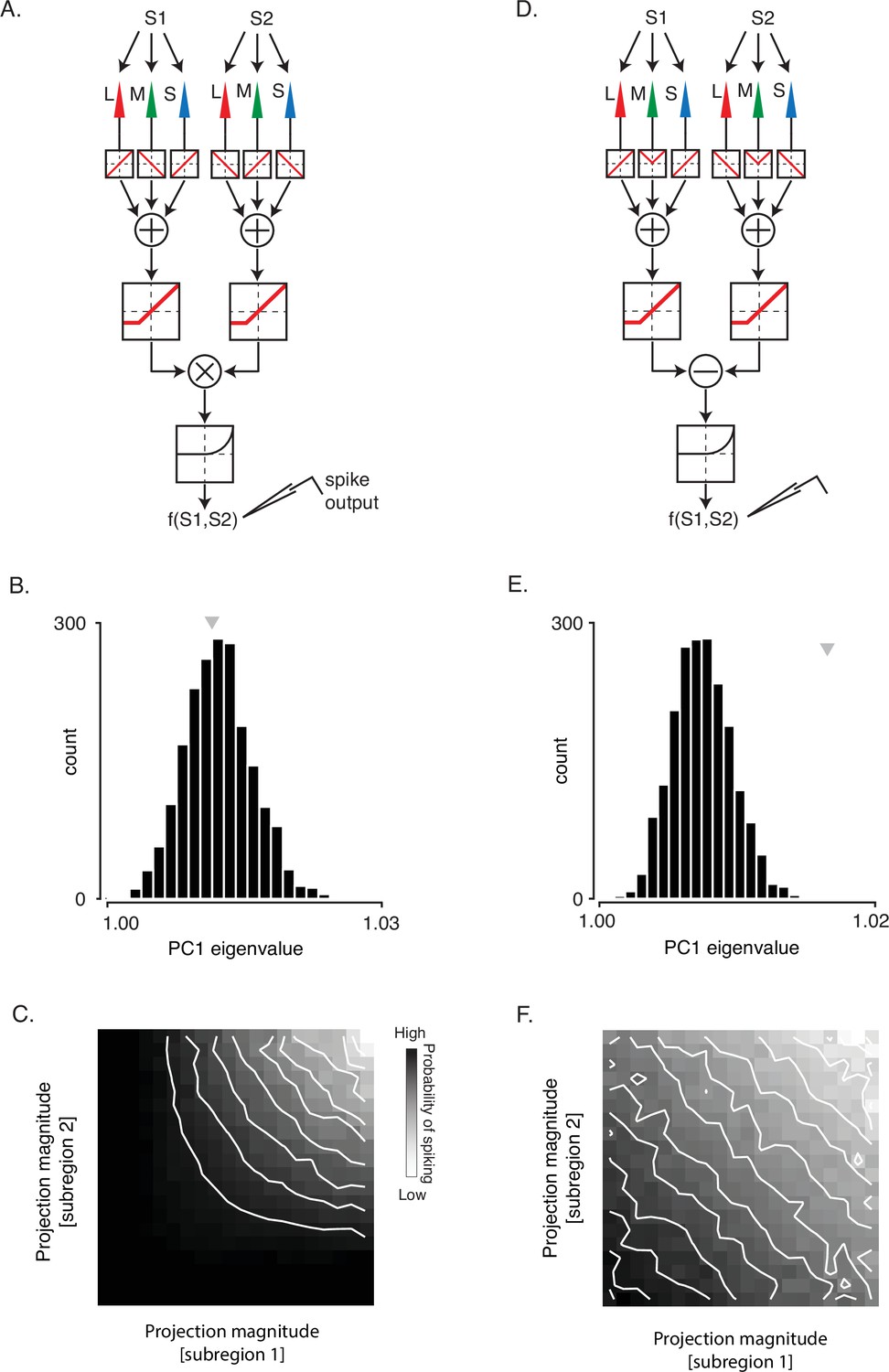
Relationship between white noise NLI and the eigenvalue corresponding to the largest principal component (PC1) for two simulated neurons.
(A) Histogram of eigenvalues obtained by randomizing time shifts between hyperpixel white noise stimuli and evoked spikes. Eigenvalue from the unrandomized data is shown as a gray triangle. In this simulation, the spiking response was given by the product of two half-wave rectified linear subfields. This nonlinearity tightens the distribution of excitatory stimuli and therefore does not manifest in the PC1. (B) A firing rate map for the simulated neuron in (A) in the same format as Figure 2C. Contours of constant spiking probability (white lines) are curved, and white noise NLI (0.028) is large, indicative of nonlinear spatial integration. (C, D). Same as (A, B) but for a simulated neuron with a half-wave rectified response to modulations of one color channel and a full-wave rectified response to another. This neuron has a large PC1 due to the full-wave rectification but a small white noise NLI (0.00) because the nonlinearity is hidden once the stimuli are projected onto the STA, which is the first step in the calculation of the white noise NLI. NLI, non-linearity index; STA, spike-triggered average.
Figure 3 with 5 supplements

Analysis of isoresponse contours.
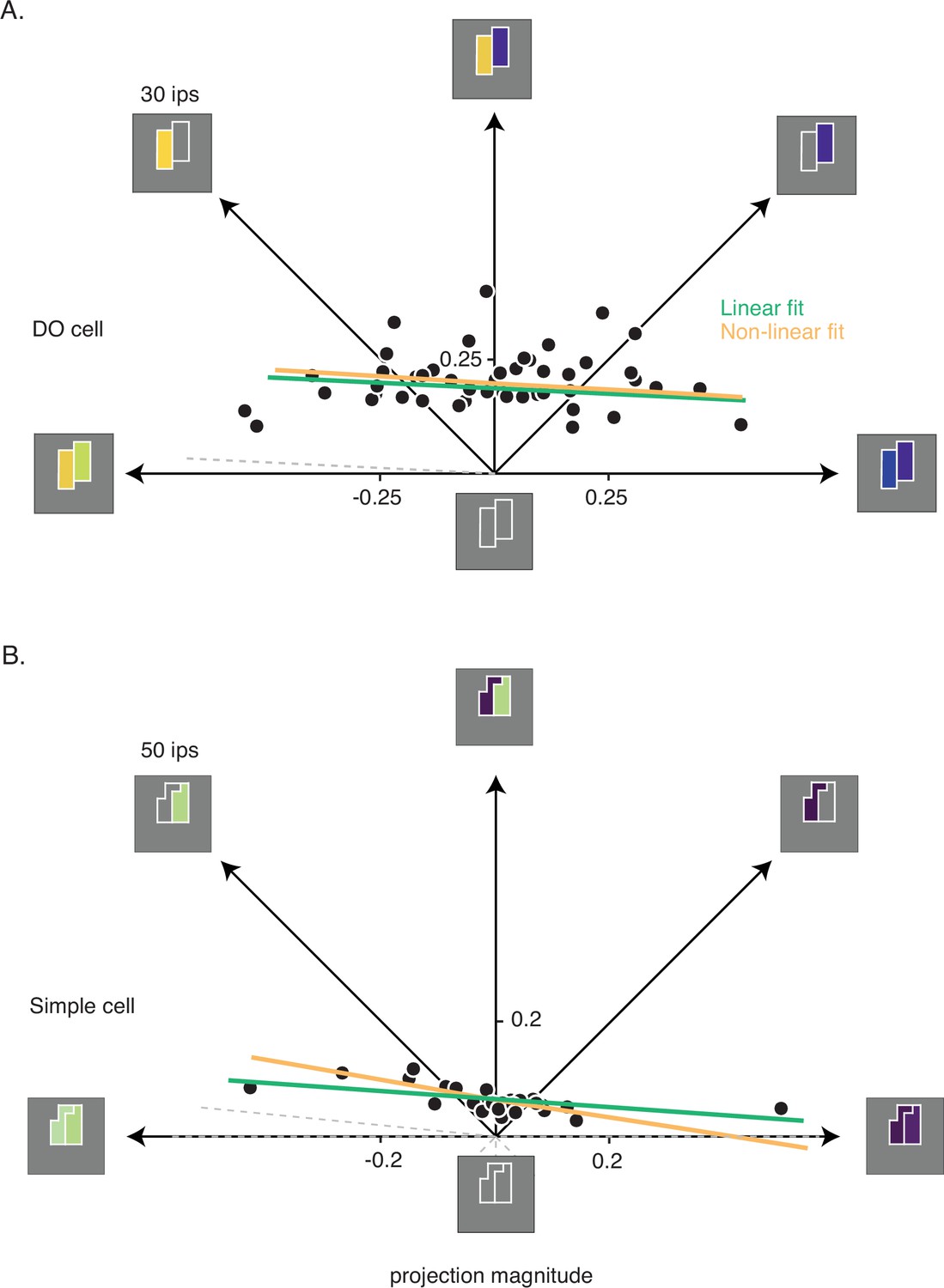
(A) Data from the example DO cell shown in Figure 2A–C. Dots indicate staircase terminations (target firing rate=30 ips) and gray dashed lines indicate staircases that exceeded the monitor gamut. Linear (green) and nonlinear (orange) fits to the data are similar. Pixel STA (to the right of the hyperpixel STA) and cone weights derived from the color weighting functions (bar plot) are also shown. (B) Same as (A) but for a simple cell (target firing rate=50 ips). L+M spectral sensitivity manifests as bright green (ON) or dark purple (OFF) when probed with RGB white noise (Chichilnisky and Kalmar, 2002). (C) Same as (A) for a cell that was spatially opponent but neither simple nor DO (target firing rate=20 ips). (D) Histogram of isoresponse NLIs. NLIs of example neurons are marked with ticks, and medians are marked with triangles. (E) Scatter plot of isoresponse NLIs and white noise NLIs. Example neurons are marked with yellow asterisks. Error bars were obtained via a jackknife procedure (see Materials and methods). DO, double-opponent; NLI, non-linearity index; STA, spike-triggered average.
Figure 3—figure supplement 1
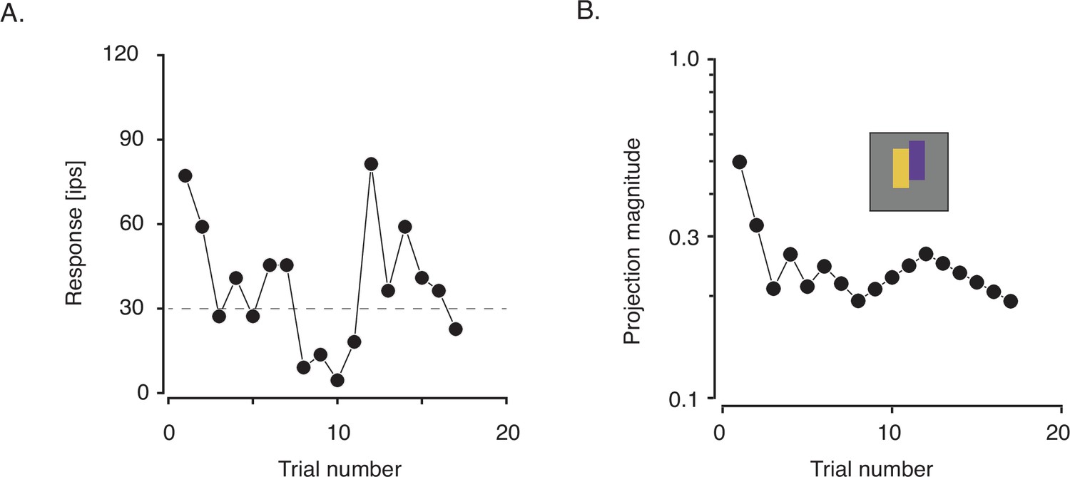
An example staircase from the closed-loop procedure used to study the DO cell in Figure 2A.
Neuronal response (in impulses per second, ips) is plotted as a function of trial number (intervening stimuli skipped). The target firing rate was 30 ips (dashed line). (B) The projection magnitude as a function of trial number for the same staircase. The staircase termination point is defined as the projection magnitude of the stimulus presented in the final (17th) trial. DO, double-opponent.
Figure 3—figure supplement 2
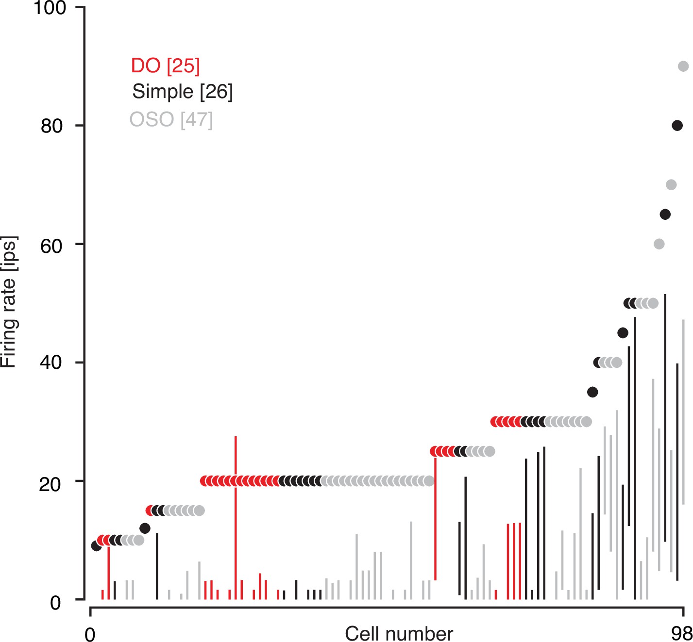
Distribution of baseline and target firing rates during Phase 3 for DO (red), simple (black), and OSO (gray) cells.
Dots indicate the target firing rates and vertical lines span the 5th to the 95th percentiles of the basline firing rate distribution. On average, the target firing rate was 15.65 standard deviations above the mean baseline firing rate. DO, double-opponent; OSO, other spatially opponent.
Figure 3—figure supplement 3
Zoomed-in isoresponse contours and staircase terminations from Figure 3A–B.
Figure 3—figure supplement 4
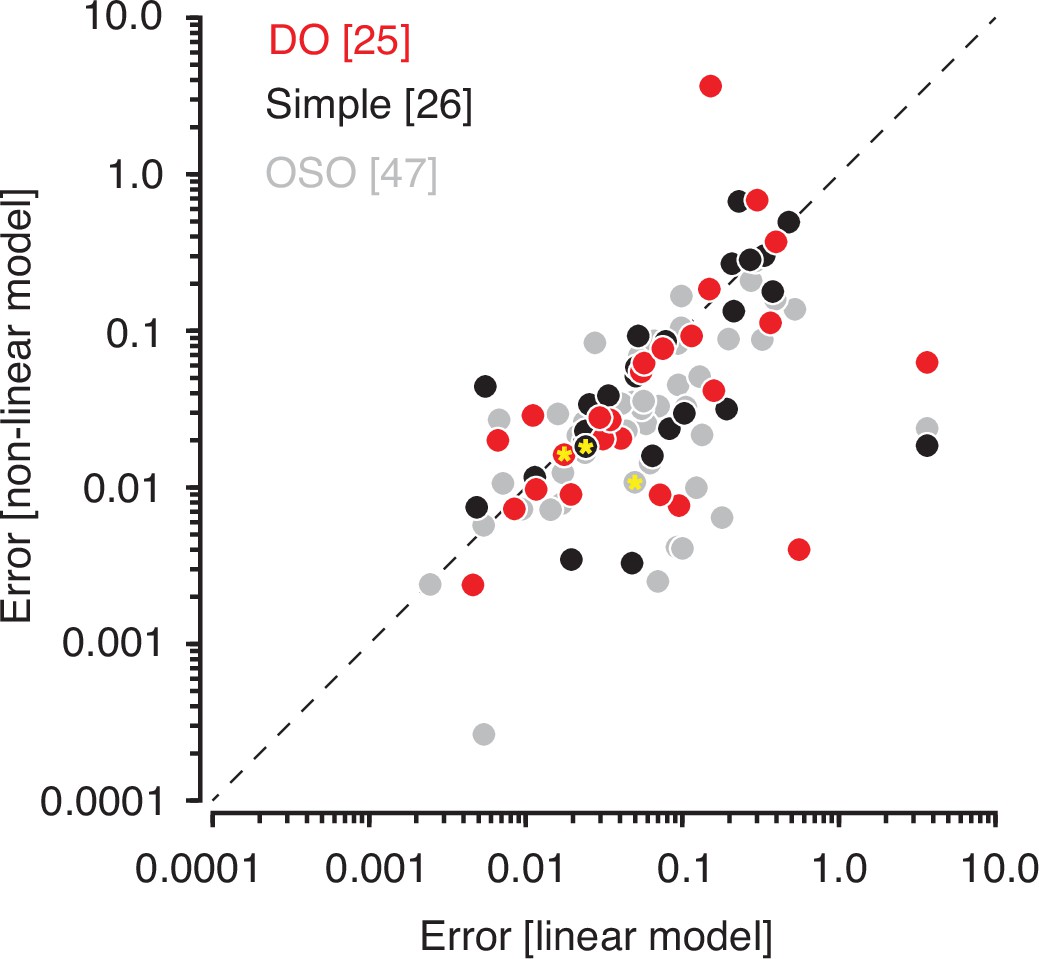
Cross-validated errors from linear (absicca) and nonlinear (ordinate) fits to data from Phase 3 for DO cells (red), simple cells (black), and OSO cells (gray).
Example neurons from Figure 3 are marked with yellow asterisks. DO, double-opponent; OSO, other spatially opponent.
Figure 3—figure supplement 5
White noise and isoresponse NLIs from neurons reclassified using alternative cone weight criteria.
A luminance tuning index was calculated for each cell by weighting and summing normalized cone weights (0.83 L+0.55 M+0.03 S). This index ranges from 0 to 1. Cells were classified as DO if their index value was <0.33 and they had an insignificant PC1. Cells were classified as simple if their index value was >0.67 and they had an insignificant PC1. Remaining cells were classified as OSO. Histograms of white noise NLIs for DO (A), simple (B), and OSO (C) cells classified this way. White noise NLIs of DO and simple cells were similar (p=0.78, Mann-Whitney U-test) and lower than those of OSO neurons (p=0.004, Mann-Whitney U-test). (D–F) Identical to (A–C) but showing isoresponse NLIs. Isoresponse NLIs for DO and simple cells were lower than for OSO neurons (p=0.06, Mann-Whitney U-test). DO, double-opponent; NLI, nonlinearity index; OSO, other spatially opponent.
Figure 4
Two models of nonlinear spatial integration.
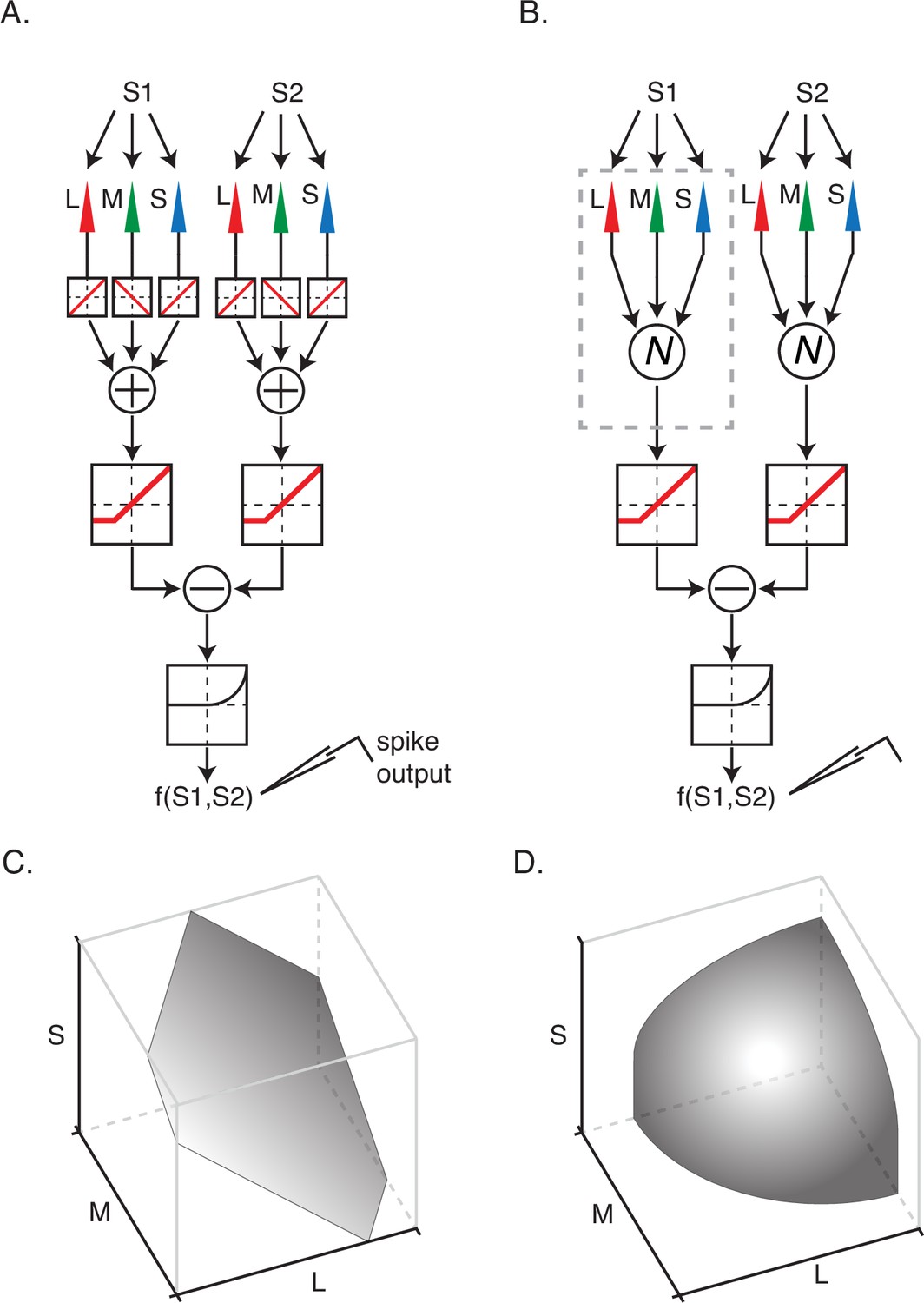
(A) A model in which signals from the three types of cone photoreceptor are integrated linearly within a subfield. The combined cone signals within each of the subunits are transformed nonlinearly and then summed to generate a response, f(S1,S2). (B) A model in which cone signals are nonlinearly transformed within a subfield prior to linear combination. (C) An isoresponse surface of firing probability is plotted as a function of cone contrasts for stimulation of a single subfield. (D) Same as (C) but for nonlinear integration model in (B). The isoresponse surface is curved in (D) and planar in (C) because signal combination within subfields is nonlinear in (B) and linear in (A).
Figure 5
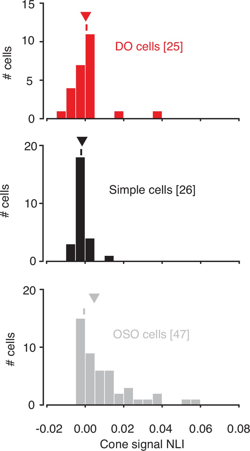
Within-subunit nonlinearity indices (NLIs) were calculated from GLMs and GQMs that predicted spikes on the basis of the RGB components of individual hyperpixels.
NLIs of example neurons in Figure 3 are marked with ticks, and medians are marked with triangles. GLM, generalized linear model; GQM, generalized quadratic model.
Figure 6
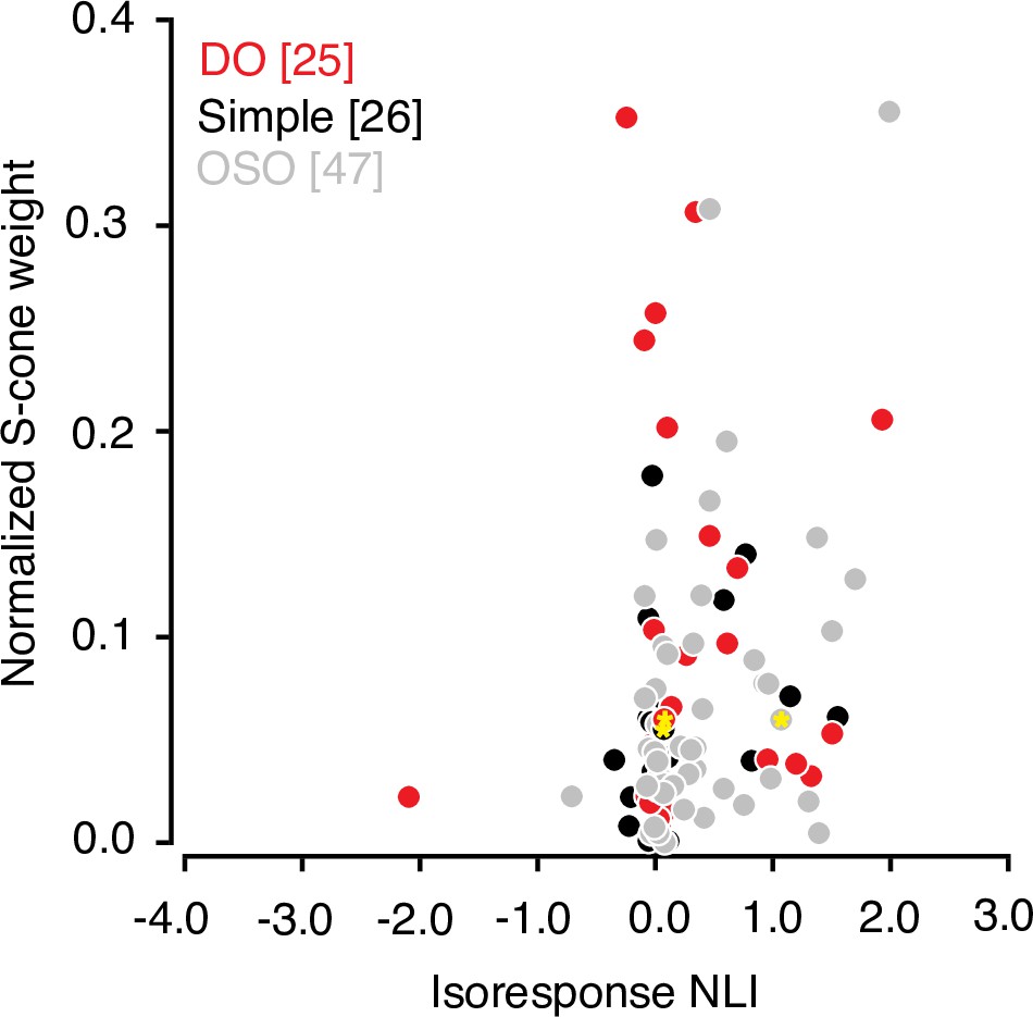
Relationship between S-cone input and signal integration across subfields.
Scatterplot of normalized S-cone weight magnitude and isoresponse NLI. Data from example neurons are marked with yellow asterisks Note that the cone weights for OSO neurons are added for the sake of completeness but must be interpreted with caution as many of the these neurons combine cone signals nonlinearly. Cone-weights are meaningful only for linear neurons. NLI, nonlinearity index; OSO, other spatially opponent.
Figure 7

Proposed signal convergence of simple cells and DO cells onto complex cells.
(A) A hypothetical complex cell receiving input from simple cells with overlapping odd- and even-symmetric receptive fields. (B) A hypothetical color-sensitive complex cell receiving input from simple and DO cells. (C) Response of a complex cell to a drifting sinusoidal grating that modulated L- and M-cones at 3 Hz with identical contrast in phase (top) and in anti-phase (bottom). (D) Same as (C) but for a color-sensitive complex cell. Gray overlays indicate stimulus duration. Both of these neurons were recorded before the hyperpixel white noise was developed and probably would have been passed over for data collection in this study because of their phase insensitivity. DO, double-opponent.
Author response image 1
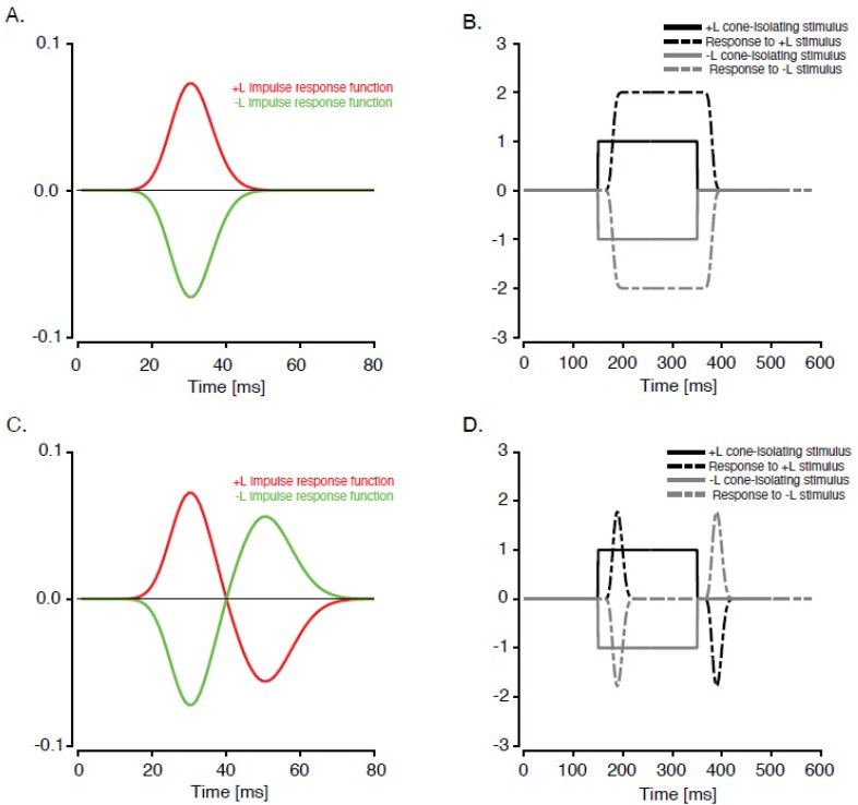
Two hypothetical, purely linear L-M neurons stimulated with L-cone isolating contrast increments and decrements.
If the temporal impulse response is monophasic (A), then the response to a step (B) is sustained, and no OFF-response occurs when the stimulus disappears. (C and D) same as A and B but for a neuron with a biphasic temporal impulse response. In this case, the disappearance of a suppressive stimulus produces an OFF response (dashed gray line).
Author response image 2
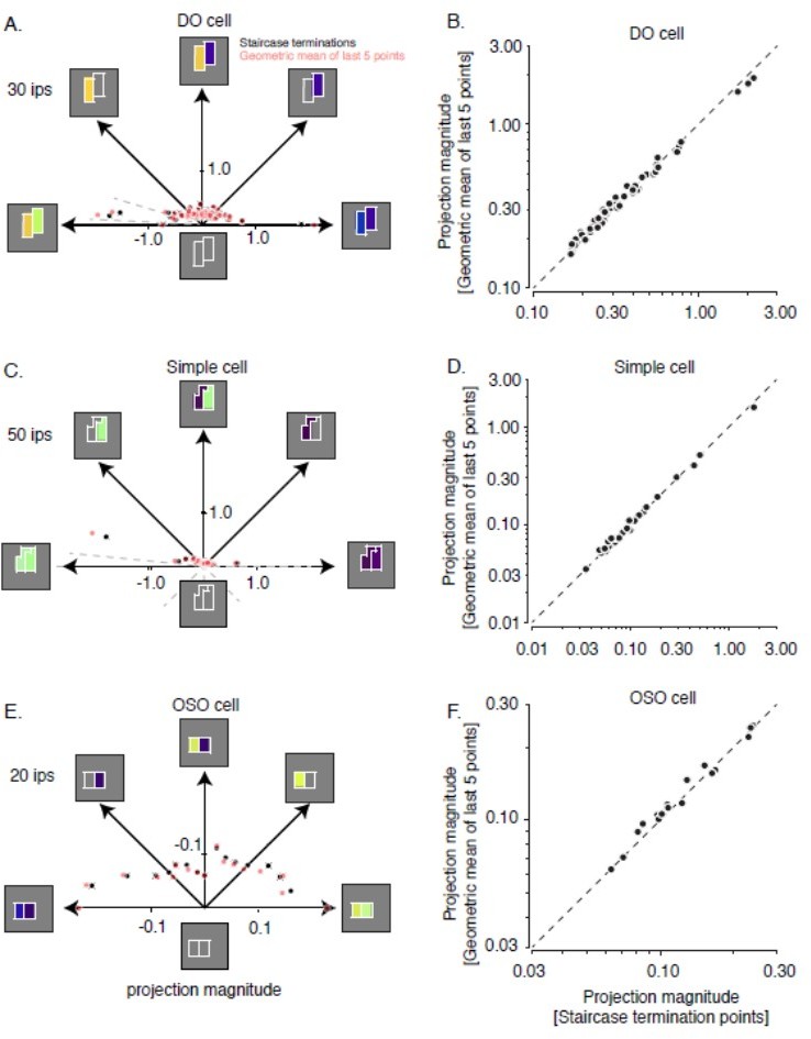
Comparison of staircase termination points with the geometric mean of the last 5 points in the staircase.
(A) Data from the example DO cell shown in Figure 3A. Black dots indicate staircase terminations and red dots indicate the geometric mean of the last 5 points in the staircase. (B) Staircase termination points are plotted against the geometric mean of the last 5 points of successful staircase terminations. (C and D) Same as A and B. but for the example simple cell shown in Figure 3B. (E and F) Same as A and B. but for the example OSO cell shown in Figure 3C.
Author response image 3
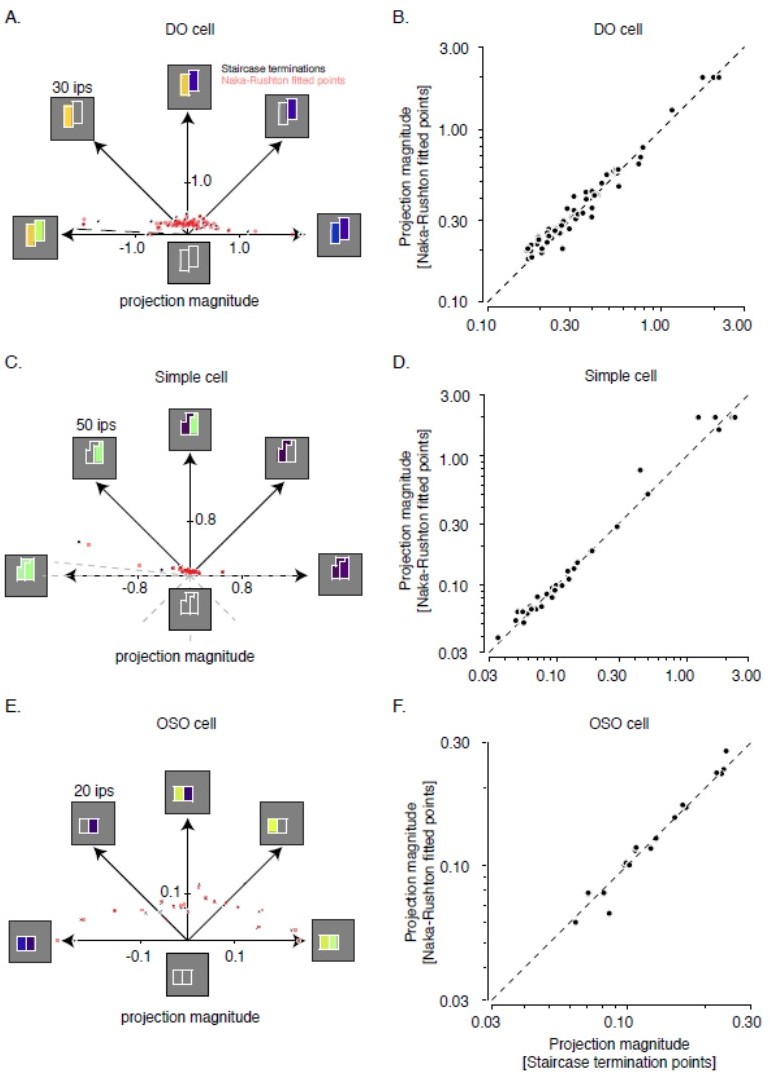
Comparison of staircase termination points with contrasts producing the target firing rate as interpolated from fitted Naka-Rushton functions.
(A) Data from the example DO cell shown in Figure 3A. Black dots indicate staircase terminations and red dots indicate Naka-Rushton fitted points. (B) Staircase termination points are plotted against the Naka Rushton fitted points. (C) and (D) same as (A) and (B) but for the example simple cell shown in Figure 3B. (E) and (F) same as (A) and (B) but for the example OSO cell shown in Figure 3C.
Tables
Key resources table
| Reagent type (species) or resource | Designation | Source or reference | Identifiers | Additional information |
|---|---|---|---|---|
| Strain, strain background (Macaca mulatta, male) | Monkey | WashingtonNational PrimateResearchCenter | Rhesus monkey | |
| Software, algorithm | Matlab | Mathworks | https://www.mathworks.com/products/matlab.html RRID:SCR_001622 | |
| Software, algorithm | Sort Client | Plexon | http://www.plexon.comRRID:SCR_003170 | |
| Software, algorithm | Offline Sorter | Plexon | http://www.plexon.comRRID:SCR_000012 |
Additional files
Download links
A two-part list of links to download the article, or parts of the article, in various formats.
Downloads (link to download the article as PDF)
Open citations (links to open the citations from this article in various online reference manager services)
Cite this article (links to download the citations from this article in formats compatible with various reference manager tools)
Coding of chromatic spatial contrast by macaque V1 neurons
eLife 11:e68133.
https://doi.org/10.7554/eLife.68133


