Increasing stimulus similarity drives nonmonotonic representational change in hippocampus
- Department of Psychology, Yale University, United States
- Department of Psychology, Queen’s University, Canada
- Department of Psychology, Princeton University, United States
- Princeton Neuroscience Institute, Princeton University, United States
Figures
Figure 1

Explanation of why moderate levels of visual similarity lead to differentiation.
Inset (bottom left) depicts the hypothesized nonmonotonic relationship between coactivation of memories and representational change from pre- to post-learning in the hippocampus. Low coactivation leads to no representational change, moderate coactivation leads to differentiation, and high coactivation leads to integration. Network diagrams show activity patterns in high-level visual cortex and the hippocampus evoked by two stimuli (A and B) with a moderate level of visual similarity that are presented as a ‘pair’ in a statistical learning procedure (such that B is reliably presented after A). Note that the hippocampus is hierarchically organized into a layer of perceptual conjunction units that respond to conjunctions of visual features and a layer of context units that respond to other features of the experimental context (McKenzie et al., 2014). Before statistical learning (left-hand column), the hippocampal representations of A and B share a context unit (because the items appeared in a highly similar experimental context) but do not share any perceptual conjunction units. The middle column (top) diagram shows network activity during statistical learning, when the B item is presented immediately following an A item; the key consequence of this sequencing is that there is residual activation of A’s representation in visual cortex when B is presented. The colored arrows are meant to indicate different sources of input converging on the unique part of each item’s hippocampal representation (in the perceptual conjunction layer) when the other item is presented: green = perceptual input from cortex due to shared features (this is proportional to the overlap in the visual cortex representations of these items); orange = recurrent input within the hippocampus; purple = input from residual activation of the unique features of the previously-presented item. The purple input is what is different between the pre-statistical-learning phase (where A is not reliably presented before B) and the statistical learning phase (where A is reliably presented before B). In this example, the orange and green sources of input are not (on their own) sufficient to activate the other item’s hippocampal representation during the pre-statistical-learning phase, but the combination of all three sources of input is enough to moderately activate A’s hippocampal representation when B is presented during the statistical learning phase. The middle column (bottom) diagram shows the learning that will occur as a result of this moderate activation, according to the NMPH: The connection between the (moderately activated) item-A hippocampal unit and the (strongly activated) hippocampal context unit is weakened (note that this is not the only learning predicted by the NMPH in this scenario, but it is the most relevant learning and hence is highlighted in the diagram). As a result of this weakening, when item A is presented after statistical learning (right-hand column, top), it does not activate the hippocampal context unit, but item B still does (right-hand column, bottom), resulting in an overall decrease in the overlap of the hippocampal representations of A and B from pre-to-post learning.
Figure 2 with 2 supplements
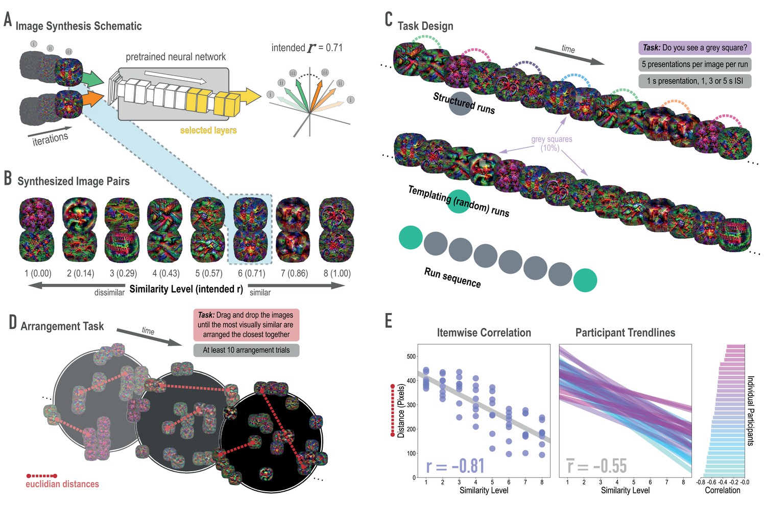
Schematic of image synthesis algorithm, fMRI task design, and behavioral validation.
(A) Our image synthesis algorithm starts with two visual noise arrays that are updated through many iterations (only three are depicted here: i, ii, and iii), until the feature activations from selected neural network layers (shown in yellow) achieve an intended Pearson correlation (r) value. (B) The result of our image synthesis algorithm was eight image pairs, that ranged in similarity from completely unrelated (similarity level 1, intended r among higher-order features = 0) to almost identical (similarity level 8, intended r = 1.00). (C) An fMRI experiment was conducted with these images to measure neural similarity and representation change. Participants performed a monitoring task in which they viewed a sequence of images, one at a time, and identified infrequent (10% of trials) gray squares in the image. Unbeknownst to participants, the sequence of images in structured runs contained the pairs (i.e. the first pairmate was always followed by the second pairmate); the images in templating runs were pseudo-randomly ordered with no pairs, making it possible to record the neural activity evoked by each image separately. (D) A behavioral experiment was conducted to verify that these similarity levels were psychologically meaningful. Participants performed an arrangement task in which they dragged and dropped images in a workspace until the most visually similar images were closest together. From the final arrangements, pairwise Euclidean distances were calculated as a measure of perceived similarity. (E) Correlation between model similarity level and distance between images (in pixels) in the arrangement task. On the left, each point represents a pair of images, with distances averaged across participants. In the center, each trendline represents the relationship between similarity level and an individual participants’ distances. The rightmost plot shows the magnitude of the correlation for each participant.
Figure 2—figure supplement 1
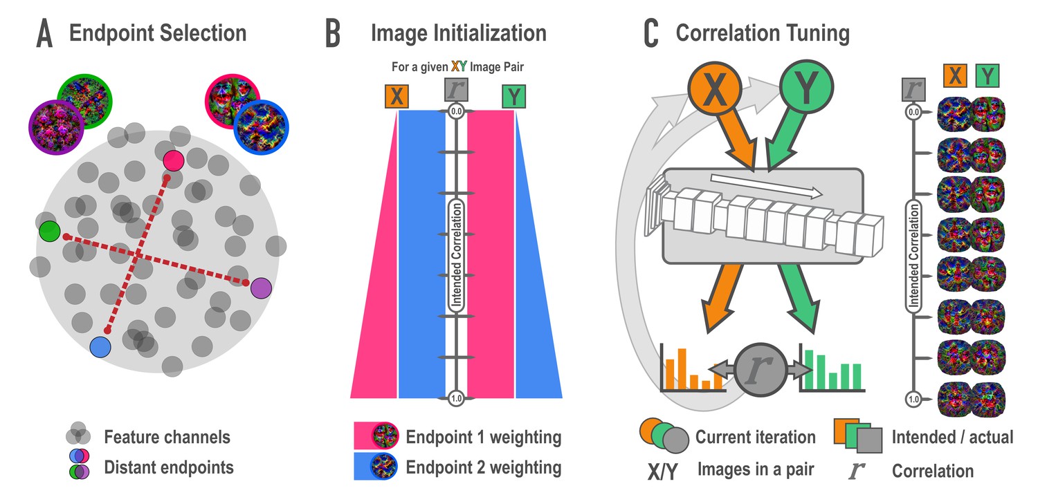
Schematic of synthesis algorithm, related to Figure 2A.
(A) In the endpoint selection phase, images were generated that maximally express each of the feature channels in a later layer of a deep neural network. These feature activations were then correlated across images and pairs of endpoint channels with the lowest possible correlation were selected. Gray circles represent feature channels and closer proximity denotes higher correlations. Colored circles highlight examples of distant, low-correlation channel pairs. (B) In the image initialization phase, paired channels served as endpoints for a weighted optimization procedure. For each endpoint pair, eight new pairs of images were created with the intention that the correlation among pairmates would span a correlation of 0 (top) to 1 (bottom) across the eight pairs. The image pairs began as simple visual noise arrays. Each image pairmate had its own endpoint, which was always maximally optimized. The other image pairmate’s endpoint was weighted according to the intended correlation. The pixels in the visual noise arrays were iteratively updated to meet this weighted goal, creating intermediate images which proceeded to the next phase. (C) In the correlation tuning phase, the feature activations for the two intermediate images of a pair were extracted from the 12 layers of interest. The correlation between these activations was computed at each iteration. The absolute difference between the intended correlation and the current iteration’s correlation was used to iteratively update the images to minimize this difference. For a single set of endpoints, image pairs were made at various intended correlations (eight shown here).
Figure 2—figure supplement 2
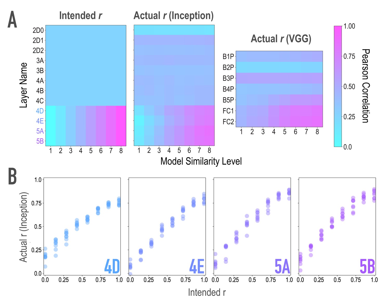
Model validation, related to Figure 2A,B.
To ensure that our model-based synthesis approach was effective in constraining the shared features among image pairs, we fed the final image pairs (Figure 1B) back through the neural network that generated them (GoogleNet/Inception; Szegedy et al., 2015; middle), as well as through an additional architecture (VGG19; Simonyan and Zisserman, 2014; right) to ensure that the similarity space produced was not dependent on the characteristics of one specific model. We extracted features from these networks for each of the generated images, and computed representational similarity matrices (RSMs) at the targeted layers to ensure that they reflected the intended similarity space. (A) Intended (left) and actual (center) correlations (r) of features across paired images as a function of similarity level and layer of the Inception model. We aimed for and achieved uniform correlations across pairs in lower and middle layers (2D0-4C), and linearly increasing correlations across pairs in higher layers (4D-5B, see panel B). Also shown are the actual feature correlations across layers of the alternate VGG19 model (right). In this alternate architecture (VGG19), the three highest model layers (B5P-FC2) mirrored the intended similarity for the highest model layers in the generating network (r(62) = 0.861, 0.849, 0.856 for the three highest model layers). The four low/middle layers (B1P-B4P) did as well (r(62) = 0.592, 0.542, 0.396, 0.455 for the four low/middle layers), but to a lesser extent (Steiger test ps < .001), and with lower variability across pairs (SD = 0.050, 0.017, 0.025, 0.052 for the four low/middle layers; for comparison, for the three highest layers: 0.116, 0.164, 0.169). (B) Comparison of feature correlations in each of the targeted higher layers of Inception (4D-5B). In the four highest layers (4D-5B), across all eight pairs of each of the eight endpoint axes (64 pairs total), the intended and actual feature correlations were strongly associated (r(62) = 0.970, 0.983, 0.977, 0.985, respectively, for the four highest layers). Considering each endpoint axis separately, the minimum feature correlations across the eight pairs of that axis remained high (r(6) = 0.945, 0.965, 0.966, 0.967, respectively, for the four highest layers). In the lower and middle layers (2D0-4C), feature correlations did not vary across pairs. This cannot be quantified by relating intended and actual feature correlations, given the lack of variance in intended feature correlations across pairs. Instead, the average differences between any two pairs in these eight lower/middle layers were small (M = 0.012, 0.011, 0.012, 0.041, 0.025, 0.045, 0.043, 0.053 for the eight lower/middle layers; for comparison, for the four highest layers M = 0.14, 0.19, 0.22, 0.23). The standard deviations of the feature correlations across pairs in these layers were also low (SD = 0.010, 0.010, 0.011, 0.035, 0.022, 0.039, 0.039, 0.048 for the eight lower/middle layers; for comparison, for the highest four layers SD = 0.199, 0.244, 0.259, 0.243).
Figure 3 with 2 supplements
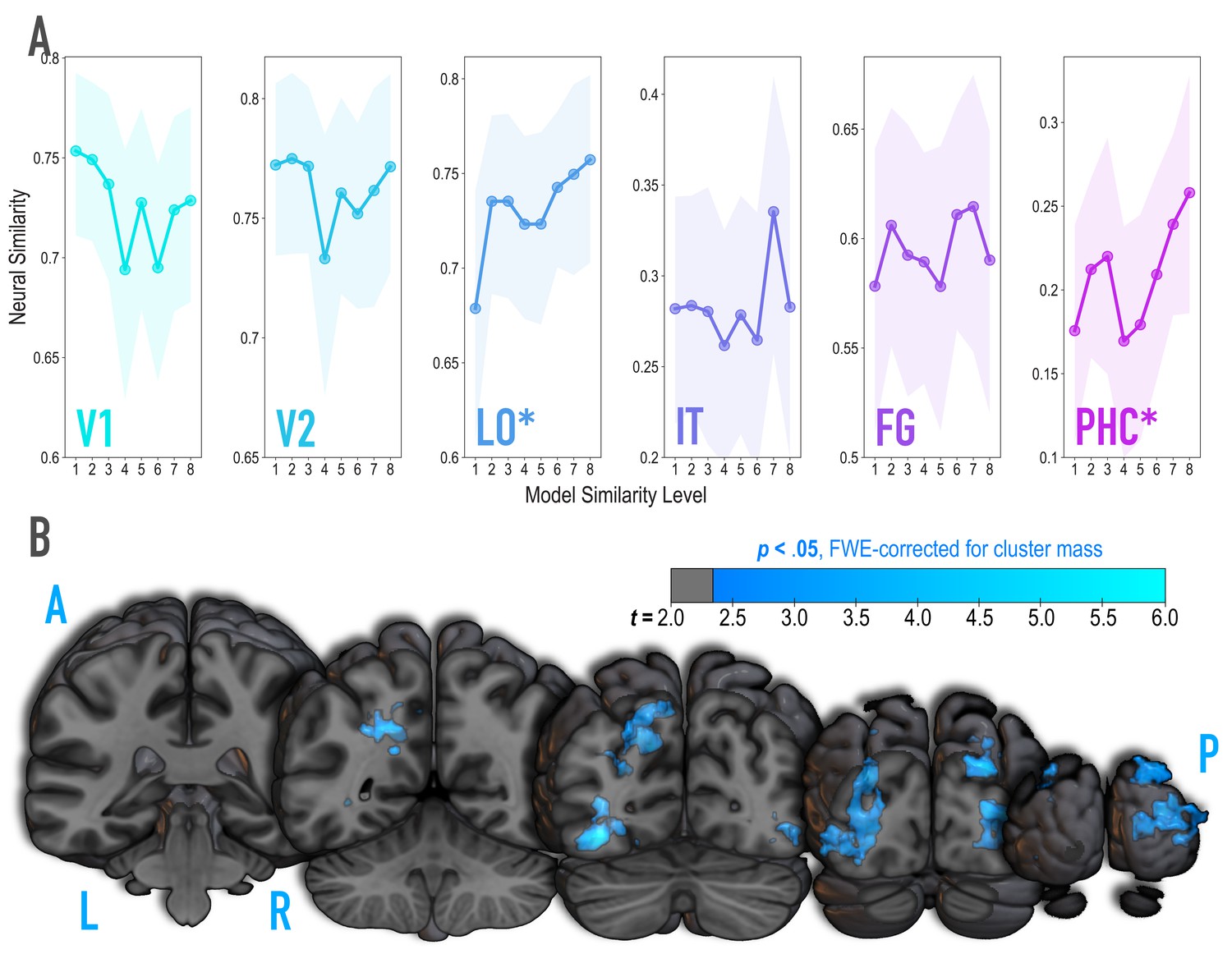
Analysis of where in the brain representational similarity tracked model similarity, prior to statistical learning.
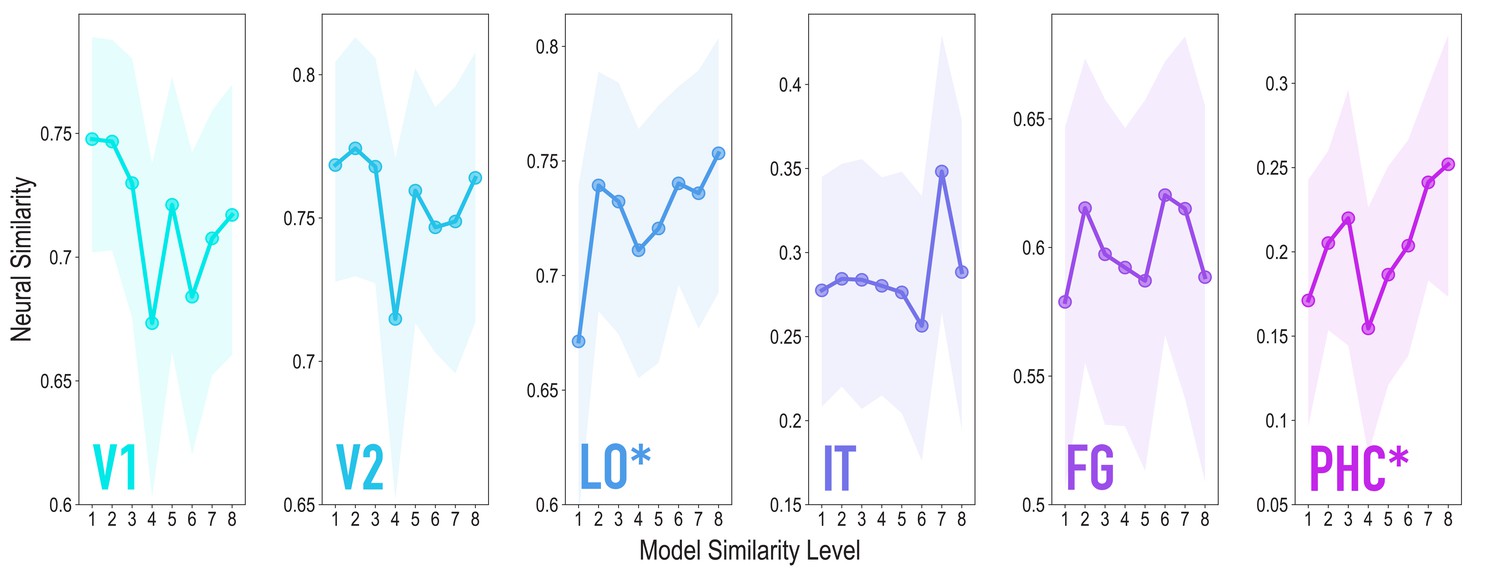
(A) Correlation of voxel activity patterns evoked by pairs of stimuli (before statistical learning) in different brain regions of interest, as a function of model similarity level (i.e. how similar the internal representations of stimuli were in the targeted layers of the model). Neural similarity was reliably positively associated with model similarity level only in LO and PHC. Shaded areas depict bootstrap resampled 95% confidence intervals at each model similarity level. (B) Searchlight analysis. Brain images depict coronal slices viewed from a posterior vantage point. Clusters in blue survived correction for family-wise error (FWE) at p < 0.05 using the null distribution of maximum cluster mass. L = left hemisphere, R = right hemisphere, A = anterior, P = posterior.
Figure 3—figure supplement 1
Similarity tracked model similarity prior to statistical learning, related to Figure 3.
Correlation of voxel activity patterns evoked by pairs of stimuli (before statistical learning) in different brain regions of interest, as a function of model similarity level (i.e. how similar the internal representations of stimuli were in the targeted layers of the model). Shaded areas depict bootstrap resampled 95% confidence intervals at each model similarity level. The pattern of results was identical to that in the full sample: model similarity level was positively associated with neural similarity in LO (mean r = 0.163, 95% CI = [0.056 0.270], randomization p = 0.024) and PHC (mean r = 0.127, 95% CI = [0.016 0.239], p = 0.031). No other region showed a significant positive relationship to model similarity (V2: mean r = −0.046, 95% CI = [−0.163 0.069], p = 0.720; IT: r = 0.090, 95% CI = [−0.049 0.226], p = 0.095; FG: r = 0.058, 95% CI = [−0.059 0.179], p = 0.195); V1 showed a negative relationship (mean r = −0.141, 95% CI = [−0.261 −0.025], p = 0.020). We also repeated the searchlight analysis in the reduced sample size, which yielded a very similar statistical map to the full sample (r = 0.928), though the clusters reported for the full sample did not survive correction.
Figure 3—figure supplement 2
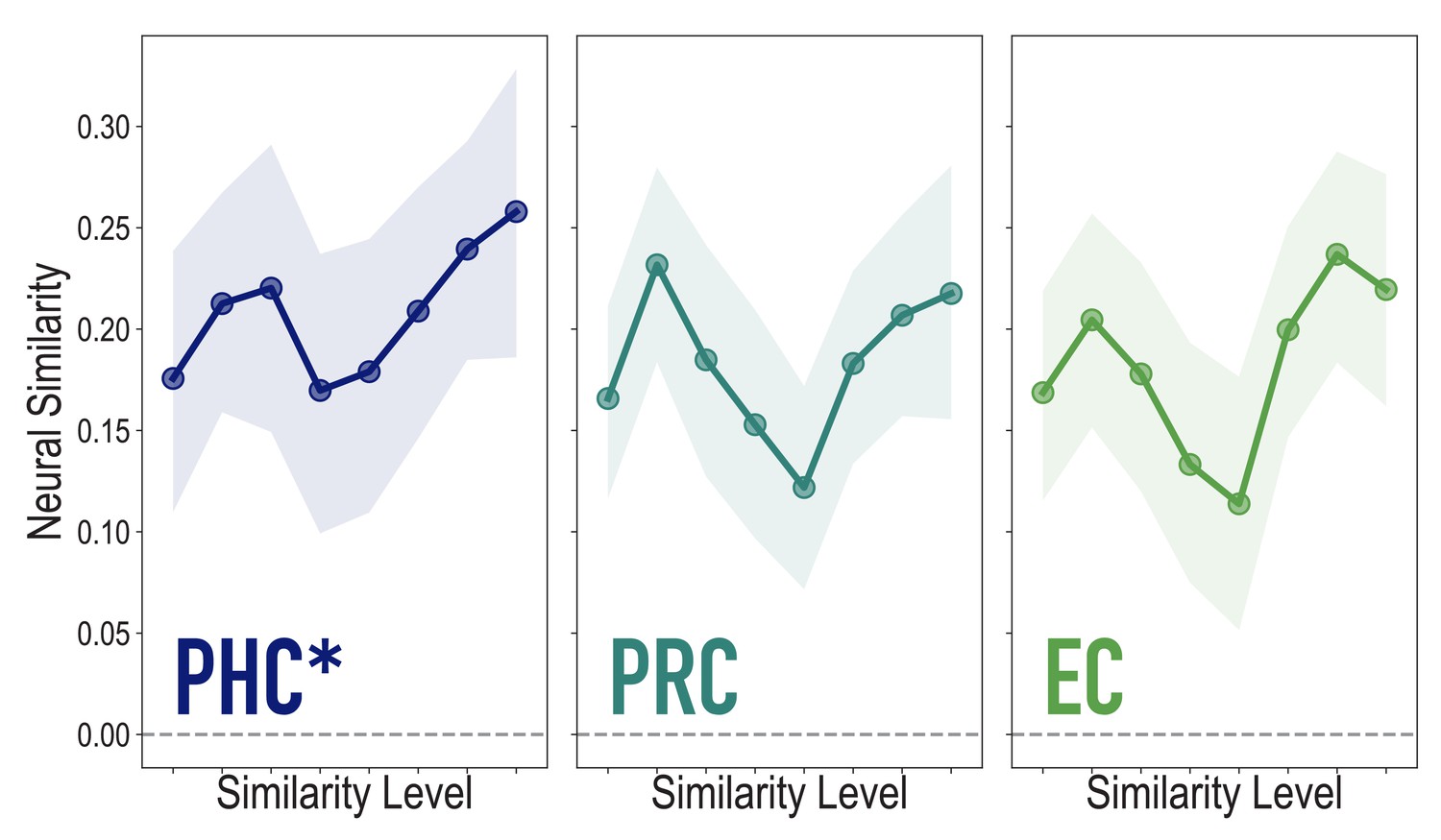
Analyses of medial temporal cortex subregions, showing neural similarity (prior to statistical learning) as a function of model similarity, related to Figure 3A.
Correlation of voxel activity patterns evoked by pairs of stimuli (before statistical learning) in different brain regions of interest, as a function of model similarity level (i.e. how similar the internal representations of stimuli were in the targeted layers of the model), in parahippocampal cortex (PHC; Duplicate figure and analysis from Figure 3A), perirhinal cortex (PRC) and entorhinal cortex (EC). Of these three regions, model similarity level was positively associated with neural similarity only in PHC (mean r = 0.126, 95% CI = [0.024 0.229], p = 0.028), not in PRC (r = 0.029, 95% CI = [−0.096 0.149], p = 0.339), or EC (r = 0.076, 95% CI = [−0.038 0.189], p = 0.154). Shaded area depicts bootstrap resampled 95% CIs.
Figure 4 with 2 supplements
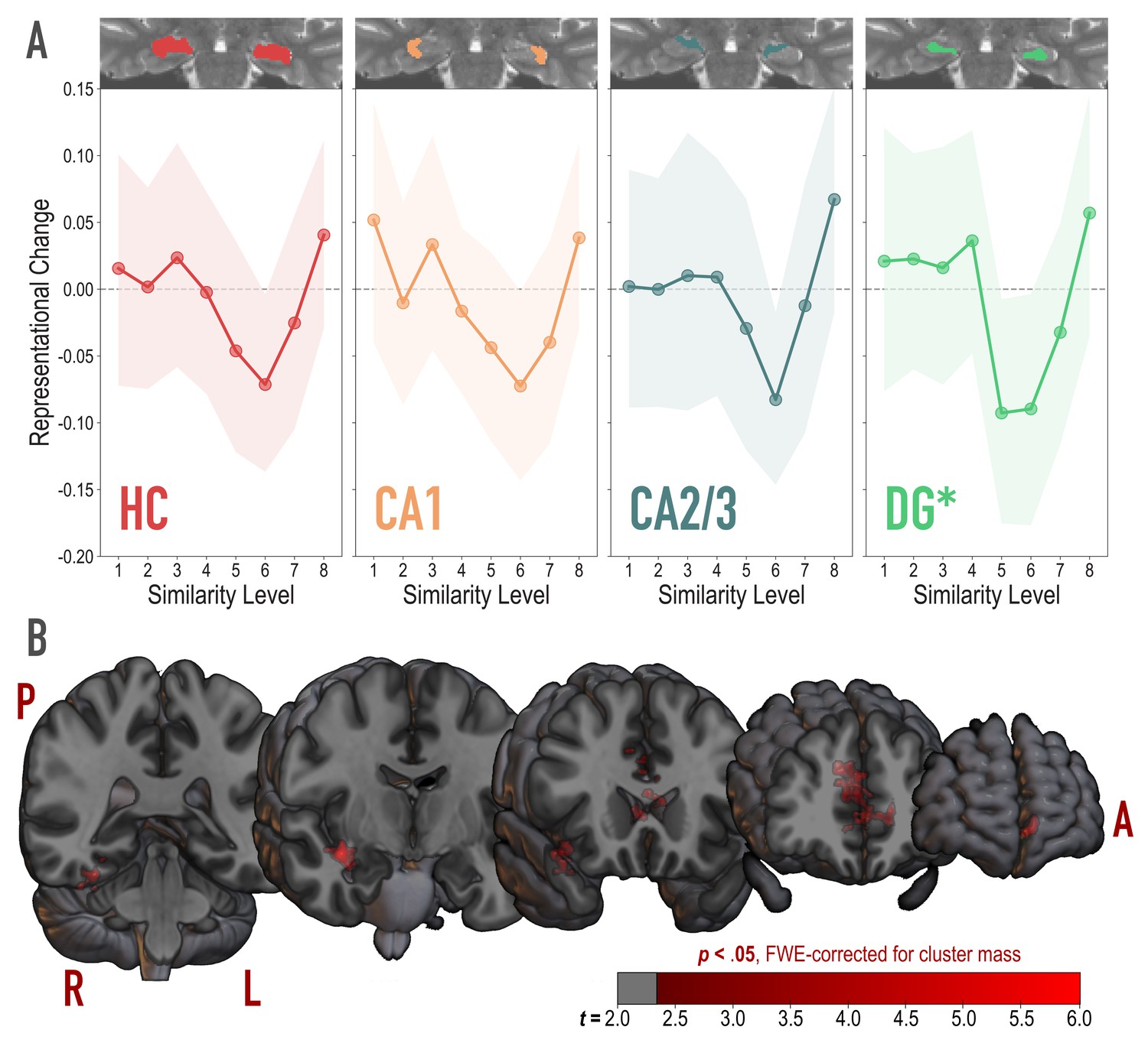
Analysis of representational change predicted by the nonmonotonic plasticity hypothesis.
(A) Difference in correlation of voxel activity patterns between paired images after minus before learning at each model similarity level, in the whole hippocampus (HC) and in hippocampal subfields CA1, CA2/3 and DG. Inset image shows an individual subject mask for the ROI in question, overlaid on their T2-weighted anatomical image. The nonmonotonic plasticity hypothesis reliably predicted representational change in DG. Shaded area depicts bootstrap resampled 95% CIs. (B) Searchlight analysis. Brain images depict coronal slices viewed from an anterior vantage point. Clusters in red survived correction for family-wise error (FWE) at p < 0.05 using the null distribution of maximum cluster mass. L = left hemisphere, R = right hemisphere, A = anterior, P = posterior.
Figure 4—figure supplement 1
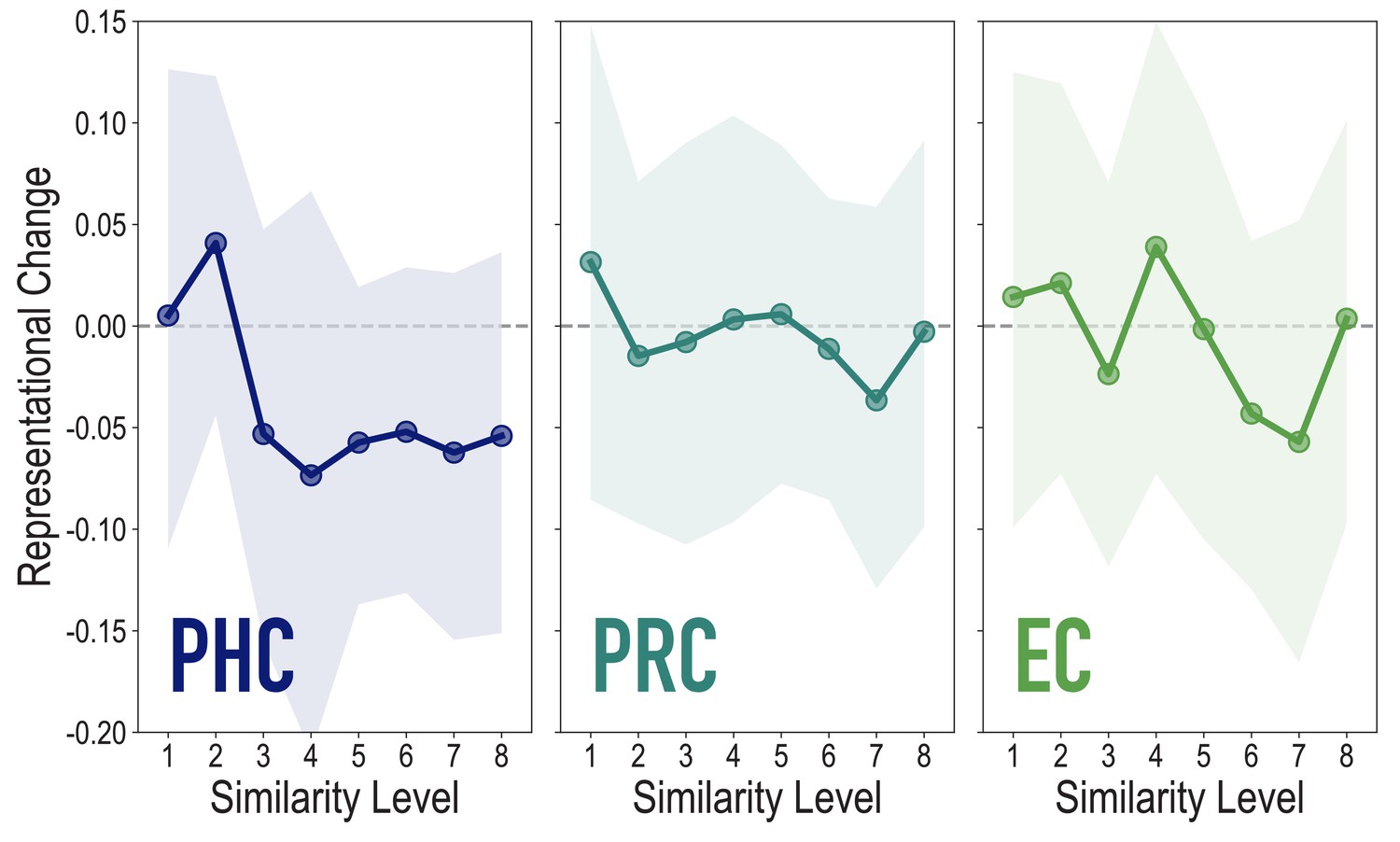
Analyses of medial temporal cortex subregions, showing representational change as a function of model similarity, related to Figure 4A.
Difference in correlation of voxel activity patterns between paired images after minus before learning at each model similarity level. Model fit was not reliable in PHC (r = 0.076, 95% CI = [−0.055 0.209], p = 0.18), PRC (r = −0.106, 95% CI = [−0.236 0.023], p = 0.79), or EC (r = −0.066, 95% CI = [−0.161 0.026], p = 0.72). Shaded area depicts bootstrap resampled 95% CIs.
Figure 4—figure supplement 2
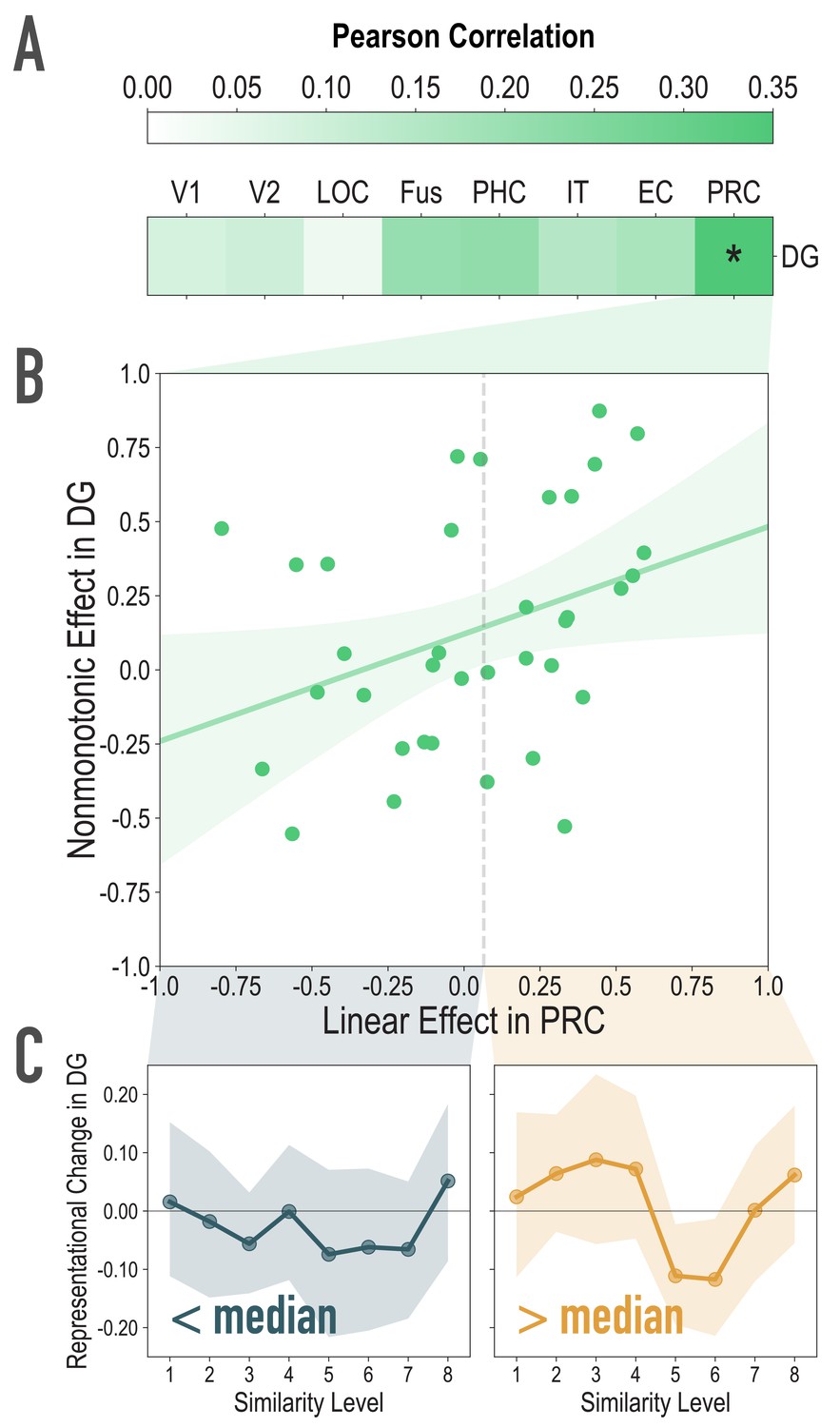
Exploratory analyses of the association between visual similarity effects in visual regions of interest, and the observed nonmonotonic effect in DG, related to Figure 4A.
(A) For each participant, we extracted the statistic for the correlation between model similarity level and representational similarity in visual regions of interest (Linear Effect), as well as the statistic for the correlation between observed representational change and predicted representational change based on the nonmonotonic model (Nonmonotonic Effect). We then probed for cortical regions where the Linear Effect was reliably associated with our observed Nonmonotonic Effect in DG. Based on bootstrap resampling participants 50000 times, the association was reliable only in PRC (mean r = 0.348, 95% CI = [0.026 0.629]). No other regions were reliably associated with the Nonmonotonic Effect in DG (V1: mean r = 0.085, 95% CI = [−0.152 0.317]; V2: mean r = 0.099, 95% CI = [−0.140 0.345]; LOC: mean r = 0.036, 95% CI = [−0.291 0.399]; Fus: mean r = 0.209, 95% CI = [−0.072 0.493]; PHC: mean r = 0.218, 95% CI = [−0.080 0.509]; IT: mean r = 0.150, 95% CI = [−0.162 0.458]; EC: mean r = 0.169, 95% CI = [−0.151 0.470]). (B) Scatterplot depicting the association between the Linear Effect in PRC and the Nonmonotonic Effect in DG. The dotted vertical gray line depicts the median Linear Effect in PRC (0.065). (C) To visualize the difference, plotted here is the difference in correlation of voxel activity patterns between paired images after minus before learning at each model similarity level in DG. The left and right plots depict participants whose Linear Effect in PRC was lower and higher than the median, respectively. Shaded area depicts bootstrap resampled 95% CIs.
Additional files
Download links
A two-part list of links to download the article, or parts of the article, in various formats.
Downloads (link to download the article as PDF)
Open citations (links to open the citations from this article in various online reference manager services)
Cite this article (links to download the citations from this article in formats compatible with various reference manager tools)
Increasing stimulus similarity drives nonmonotonic representational change in hippocampus
eLife 11:e68344.
https://doi.org/10.7554/eLife.68344


