Research Article

Neuroscience

Global organization of neuronal activity only requires unstructured local connectivity

Institute of Neuroscience and Medicine and Institute for Advanced Simulation and JARA Institut Brain Structure-Function Relationships, Jülich Research Centre, Germany
RWTH Aachen University, Germany
School of Computing, University of Leeds, United Kingdom
Institut de Neurosciences de la Timone, CNRS - Aix-Marseille University, France
Department of Physics, Faculty 1, RWTH Aachen University, Germany
Department of Psychiatry, Psychotherapy and Psychosomatics, School of Medicine, RWTH Aachen University, Germany
Theoretical Systems Neurobiology, RWTH Aachen University, Germany

Jan 20, 2022

https://doi.org/10.7554/eLife.68422

Open access
Copyright information

Figures
Tables
Additional files

13 figures, 4 tables and 1 additional file

Figures

Figure 1

Download asset Open asset

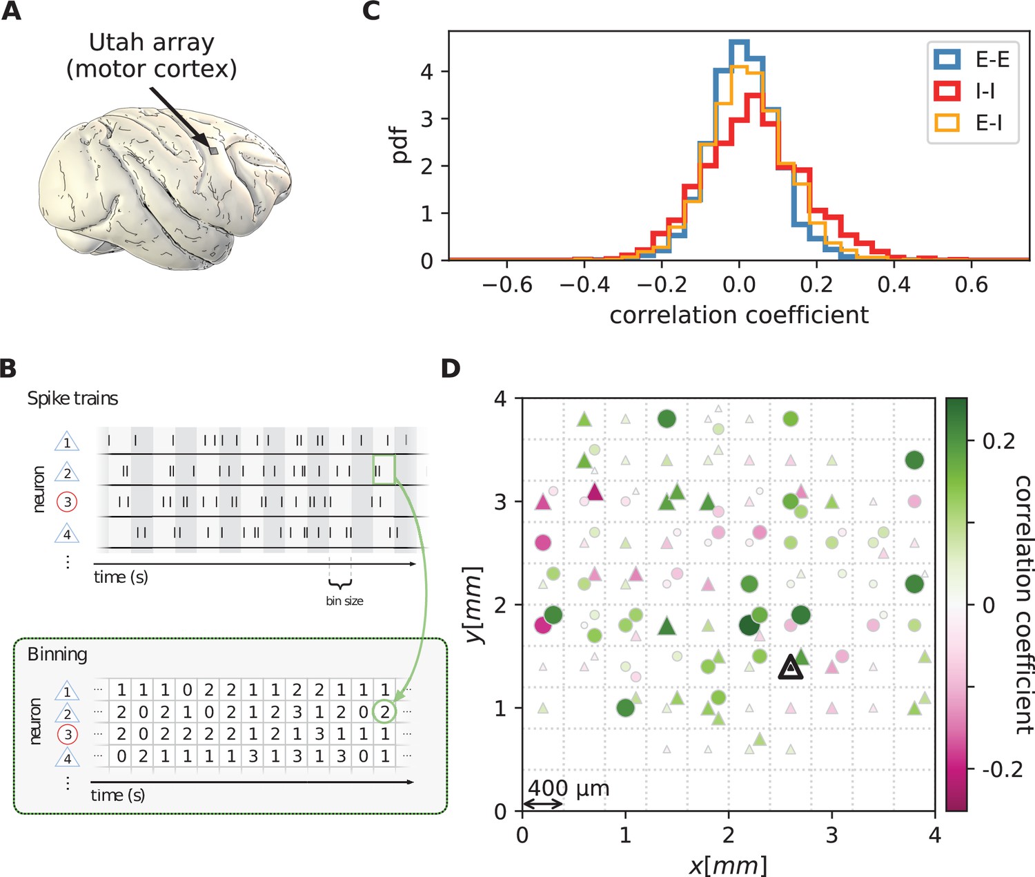
Salt-and-pepper structure of covariances in motor cortex.

(A) Sketch of 10 × 10 Utah electrode array recording in motor cortex of macaque monkey during rest. (B) Spikes are sorted into putative excitatory (blue triangles) and inhibitory (red circles) single units according to widths of spike waveforms (see Appendix 1 Section 2). Resulting spike trains are binned in 1 s bins to obtain spike counts. (C) Population-resolved distribution of pairwise spike-count Pearson correlation coefficients in session E2 (E-E: excitatory-excitatory, E-I: excitatory-inhibitory, I-I: inhibitory-inhibitory). (D) Pairwise spike-count correlation coefficients with respect to the neuron marked by black triangle in one recording (session E2, see Materials and methods). Grid indicates electrodes of a Utah array, triangles and circles correspond to putative excitatory and inhibitory neurons, respectively. Size as well as color of markers represent correlation. Neurons within the same square were recorded on the same electrode.

Figure 1—source data 1 Code and data.: https://cdn.elifesciences.org/articles/68422/elife-68422-fig1-data1-v1.zip
Download elife-68422-fig1-data1-v1.zip

Figure 2

Download asset Open asset

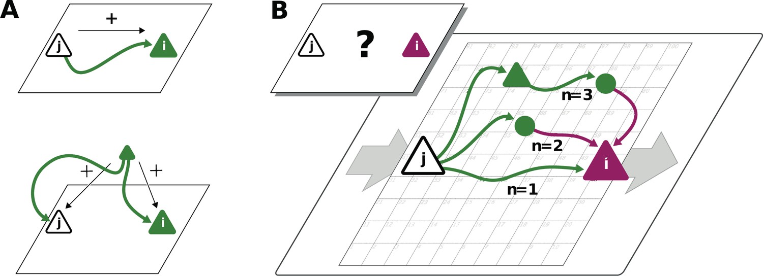
Correlations from direct and indirect connections.

(A) Positive correlation (green neuron i) follows from direct excitatory connection (top) or shared input (middle). (B) Negative correlation (magenta) between two excitatory neurons cannot be explained by direct connections: Neuronal interactions are not only mediated via direct connections ( $n = 1$ ; sign uniquely determined by presynaptic neuron type) but also via indirect paths of different length $n §gt; 1$ . The latter may have any sign (positive: green; negative: purple) due to intermediate neurons of arbitrary type (triangle: excitatory, circle: inhibitory).

Figure 3

Download asset Open asset

Spatially organized E-I network model.

(A) Network model: space is divided into cells with four excitatory (triangles) and one inhibitory (circle) neuron each. Distance-dependent connection probabilities (shaded areas) are defined with respect to cell locations. (B) Eigenvalues λ of effective connectivity matrix for network in dynamically balanced critical state. Each dot shows the real part $Re (λ)$ and imaginary part $Im (λ)$ of one complex eigenvalue. The spectral bound (dashed vertical line) denotes the right-most edge of the eigenvalue spectrum. (C) Simulation: covariances of excitatory neurons over distance $x$ between cells (blue dots: individual pairs; cyan: mean; orange: standard deviation; sample of 150 covariances at each of 200 chosen distances). (D) Theory: variance of covariance distribution as a function of distance $x$ for different spectral bounds of the effective connectivity matrix. *Inset*: effective decay constant of variances diverges as the spectral bound approaches one. (E) For large spectral bounds, the variances of EE, EI, and II covariances decay on a similar length scale. Spectral bound $R = 0.95$ . Other parameters see Appendix 1—table 3.

Figure 3—source data 1 Code and data.: https://cdn.elifesciences.org/articles/68422/elife-68422-fig3-data1-v1.zip
Download elife-68422-fig3-data1-v1.zip

Figure 4

Download asset Open asset

Long-range covariances in macaque motor cortex.

Variance of covariances as a function of distance. (A) Population-specific exponential fits (lines) to variances of covariances (dots) in session E2, with fitted decay constants indicated in the legend (I-I: putative inhibitory neuron pairs, I-E: inhibitory-excitatory, E-E: excitatory pairs). Dots show the empirical estimate of the variance of the covariance distribution for each distance. Size of the dots represents relative count of pairs per distance and was used as weighting factor for the fits to compensate for uncertainty at large distances, where variance estimates are based on fewer samples. Mean squared error 2.918. (B) Population-specific exponential fits (lines) analogous to (A), with slopes constrained to be identical. This procedure yields a single fitted decay constant of 1.029 mm. Mean squared error 2.934. (C) Table listing decay constants fitted as in (B) for all recording sessions and the ratios between mean squared errors of the fits obtained in procedures B and A.

Figure 4—source data 1 Code and data.: https://cdn.elifesciences.org/articles/68422/elife-68422-fig4-data1-v1.zip
Download elife-68422-fig4-data1-v1.zip

Figure 5

Download asset Open asset

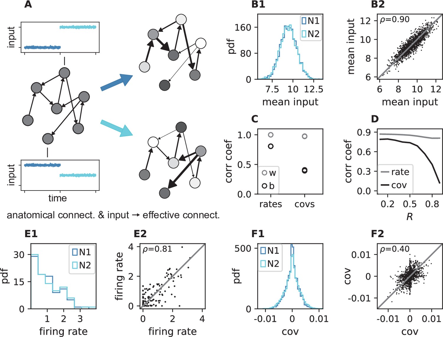
Changes in effective connectivity modify coordination patterns.

(A) Visualization of effective connectivity: A sparse random network with given structural connectivity (left network sketch) is simulated with two different input levels for each neuron (depicted by insets), resulting in different firing rates (grayscale in right network sketches) and therefore different effective connectivities (thickness of connections) in the two simulations. Parameters can be found in Appendix 1—table 4. (B1) Histogram of input currents across neurons for the two simulations (N1 and N2). (B2) Scatter plot of inputs to subset of 1500 corresponding neurons in the first and the second simulation (Pearson correlation coefficient $ρ = 0.90$ ). (C) Correlation coefficients of rates and of covariances between the two simulations (b, black) and within two epochs of the same simulation (w, gray). (D) Correlation coefficient of rates (gray) and covariances (black) between the two simulations as a function of the spectral bound $R$ . (E1) Distribution of rates in the two simulations (excluding silent neurons with $| rate | §lt; 10^{- 3}$ ). (E2) Scatter plot of rates in the first compared to the second simulation (Pearson correlation coefficient $ρ = 0.81$ ). (F1) Distribution of covariances in the two simulation (excluding silent neurons). (F2) Scatter plot of sample of 5000 covariances in first compared to the second simulation (Pearson correlation coefficient $ρ = 0.40$ ). Here silent neurons are included (accumulation of markers on the axes). Other parameters: number of neurons $N = 2000$ , connection probability $p = 0.1$ , spectral bound for panels B, C, E, F is $R = 0.8$ .

Figure 5—source data 1 Code and data.: https://cdn.elifesciences.org/articles/68422/elife-68422-fig5-data1-v1.zip
Download elife-68422-fig5-data1-v1.zip

Figure 6

Download asset Open asset

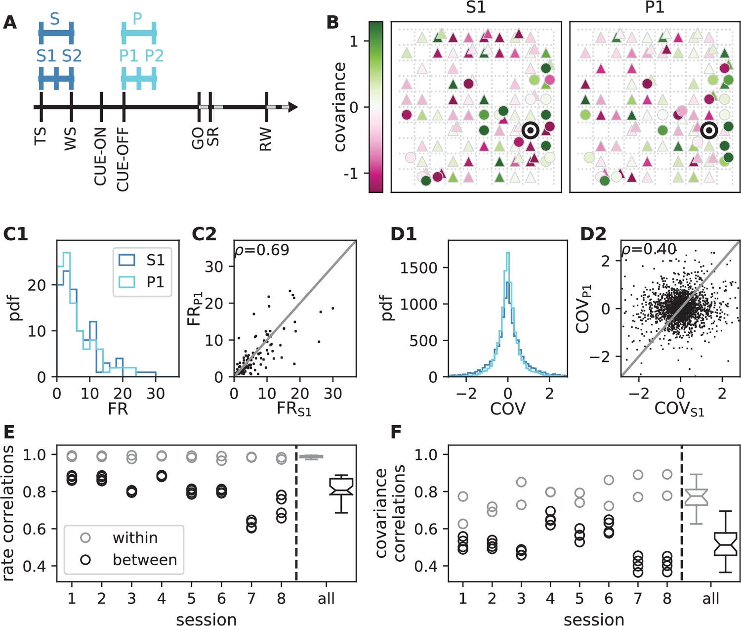
Behavioral condition reshapes mesoscopic neuronal coordination.

(A) Trial structure of the reach-to-grasp experiment (Brochier et al., 2018). Blue segments above the time axis indicate data pieces at trial start (dark blue: S (S1+ S2)) and during the preparatory period (light blue: P (P1+ P2)). (B) Salt-and-pepper structure of covariance during two different epochs (S1 and P1) of one recording session of monkey N (151 trials, 106 single units, Figure 1 for recording setup). For some neurons, the covariance completely reverses, while in the others it does not change. Inhibitory reference neuron indicated by black circle. (C1) Distributions of firing rates during S1 and P1. (C2) Scatter plot comparing firing rates in S1 and P1 (Pearson correlation coefficient $ρ = 0.69$ ). (D1/D2) Same as panels C1/C2, but for covariances (Pearson correlation coefficient $ρ = 0.40$ ). (E) Correlation coefficient of firing rates across neurons in different epochs of a trial for eight recorded sessions. Correlations between sub-periods of the same epoch (S1-S2, P1-P2; within-epoch, gray) and between sub-periods of different epochs (Sx-Py; between-epochs, black). Data shown in panels B-D is from session 8. Box plots to the right of the black dashed line show distributions obtained after pooling across all analyzed recording sessions per monkey. The line in the center of each box represents the median, box’s area represents the interquartile range, and the whiskers indicate minimum and maximum of the distribution (outliers excluded). Those distributions differ significantly (Student t-test, two-sided, $p ≪ 0.001$ ). (F) Correlation coefficient of covariances, analogous to panel E. The distributions of values pooled across sessions also differ significantly (Student t-test, two-sided, $p ≪ 0.001$ ). For details of the statistical tests, see Materials and methods. Details on number of trials and units in each recording session are provided in Appendix 1—table 1.

Figure 6—source data 1 Code and data.: https://cdn.elifesciences.org/articles/68422/elife-68422-fig6-data1-v1.zip
Download elife-68422-fig6-data1-v1.zip

Appendix 1—figure 1

Download asset Open asset

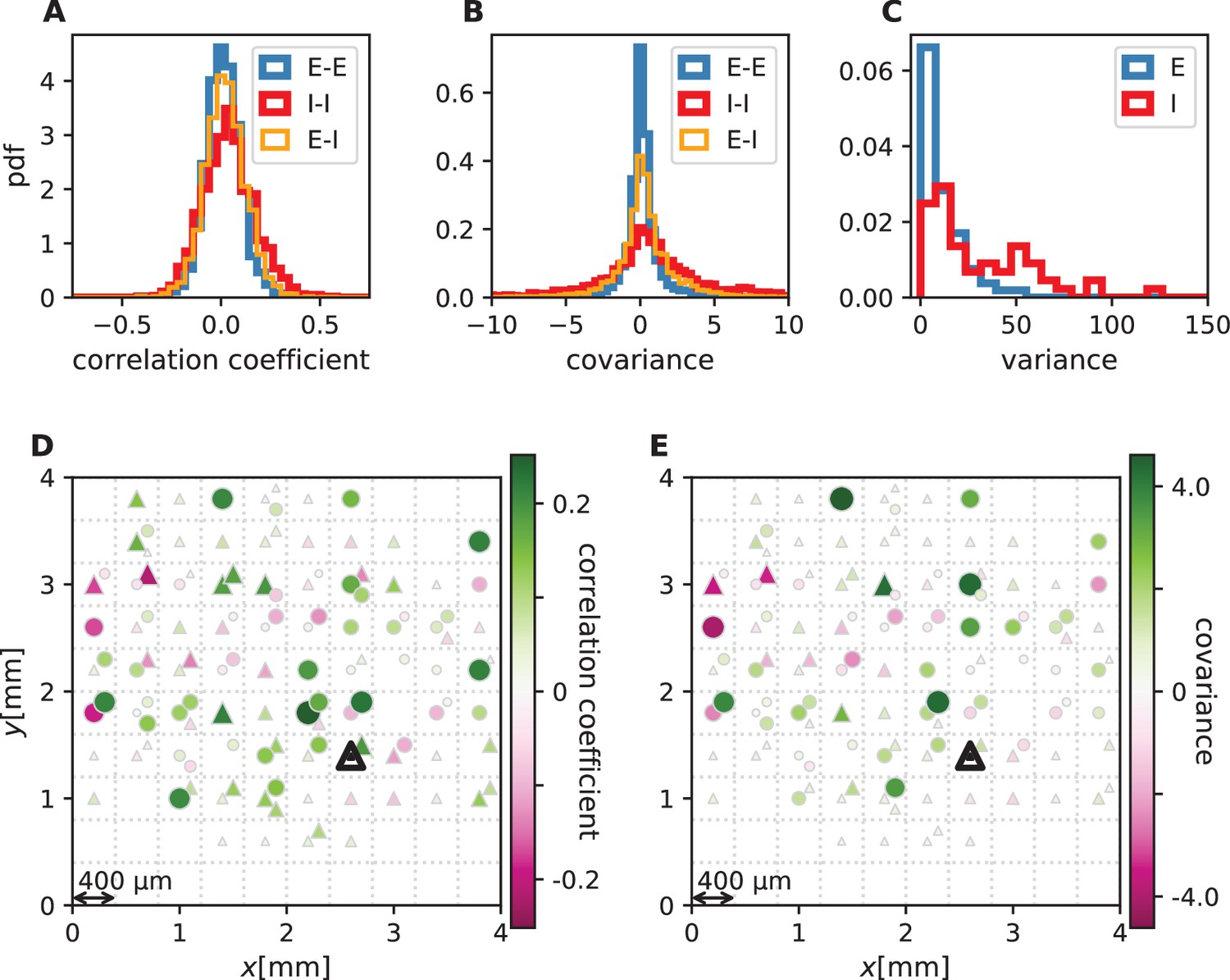
Correlations and covariances.

The shown data is taken from session E2. (E-E: excitatory-excitatory, E-I: excitatory-inhibitory, I-I: inhibitory-inhibitory). (A) Population-resolved distribution of pairwise spike-count Pearson correlation coefficients. Same data as in Figure 1C. (B) Population-resolved distribution of pairwise spike-count covariances. (C) Population-resolved distribution of variances. (D) Pairwise spike-count correlation coefficients with respect to the neuron marked by black triangle. Grid indicates electrodes of a Utah array, triangles and circles correspond to putative excitatory and inhibitory neurons, respectively. Size as well as color of markers represent correlation. Neurons within the same square were recorded on the same electrode. Same data as in Figure 1D. (E) Pairwise spike-count covariances with respect to the neuron marked by black triangle.

Appendix 1—figure 2

Download asset Open asset

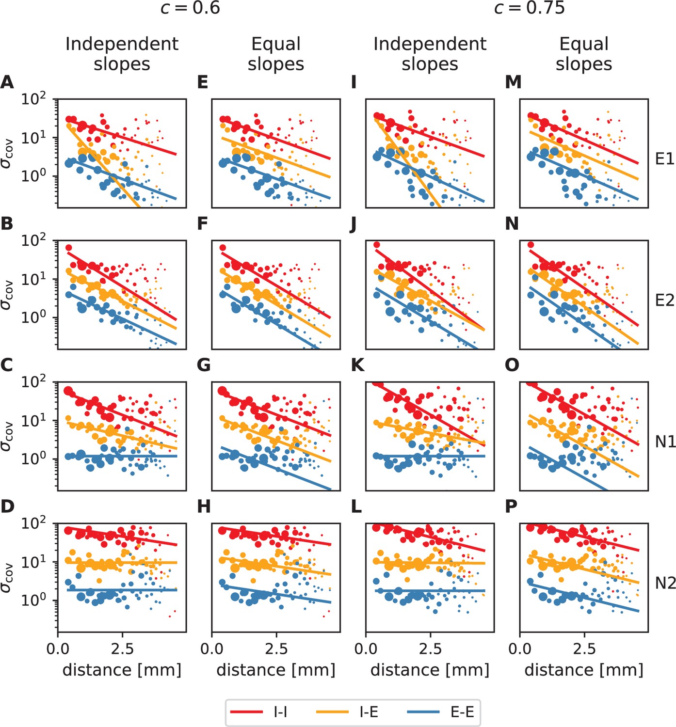
Distance-resolved variance of covariance: robustness of decay constant estimation.

Exponential fits (lines) to variances of covariances (dots) analogous to Figure 4A and B in the main text (columns 1&3 and 2&4, respectively) for all analyzed resting state sessions. The two sets of plots differ in E/I separation consistency values chosen during data preprocessing. Panels **A-H**: default (lowest) required consistency (~0.6), used throughout the main analysis; panels **I-P**: $c = 0.75$ The values of the obtained decay constants are listed in Appendix 1—table 1.

Appendix 1—figure 3

Download asset Open asset

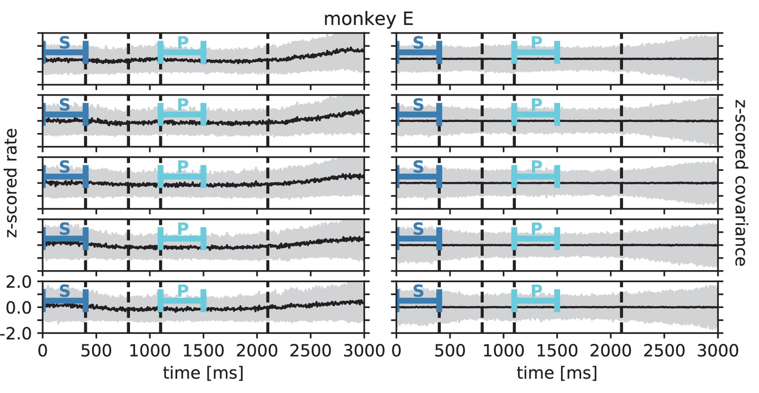
Rate and covariance stationarity during a reach-to-grasp trial: monkey E.

Black line indicates population mean and gray area +/- 1 population standard deviation of single unit firing rate (left column) and pairwise zero time-lag covariance (right column) during trial of a given session (row). Blue bars indicate starting (S) and preparatory (P) periods used in the analysis (Figure 6 in the main text). First, second and fourth dashed lines indicate visual signals lighting up and the third dashed line indicates the removal of a visual cue and beginning of a waiting period.

Appendix 1—figure 4

Download asset Open asset

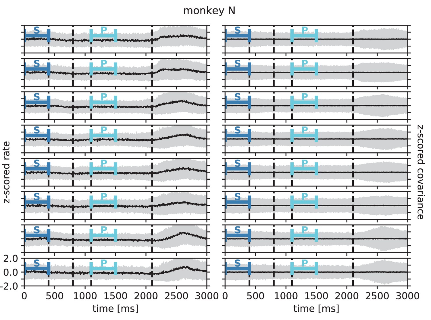
Rate and covariance stationarity during a reach-to-grasp trial: monkey N.

Analogous to Appendix 1—figure 3.

Appendix 1—figure 5

Download asset Open asset

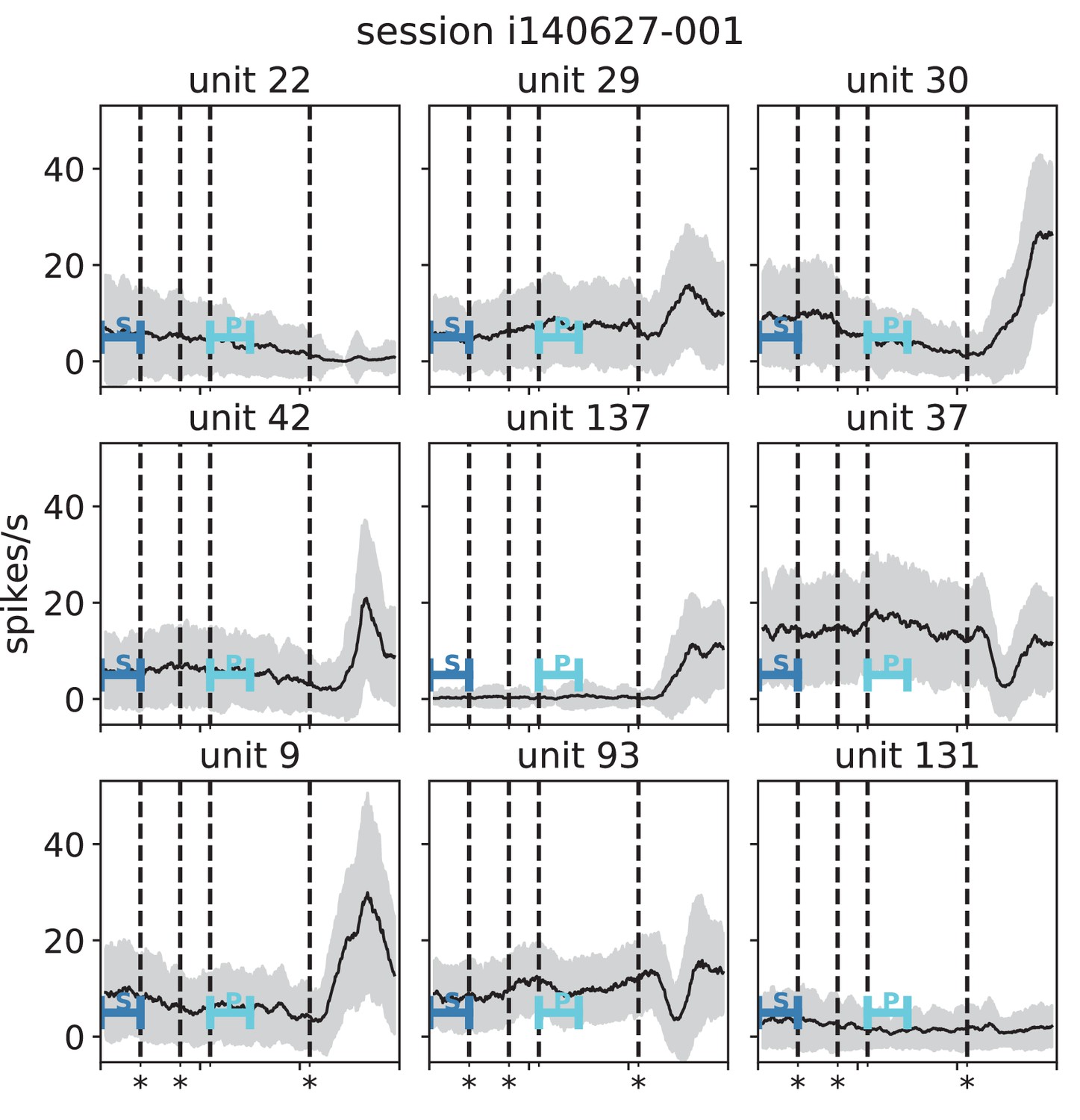
Stationarity of single-unit activity during a reach-to-grasp trial (monkey N, session i140627-001).

Black lines indicate mean and gray areas +/- 1 standard deviation across trials of single unit activity in each panel (sliding window analysis with 5 ms step size and 100 ms window length). Blue bars indicate starting (S) and preparatory (P) periods used in the analysis (Figure 6 in the main text). First, second and fourth dashed lines (marked with stars) indicate visual signals lighting up and the third dashed line indicates the removal of a visual cue and beginning of a waiting period.

Appendix 1—figure 6

Download asset Open asset

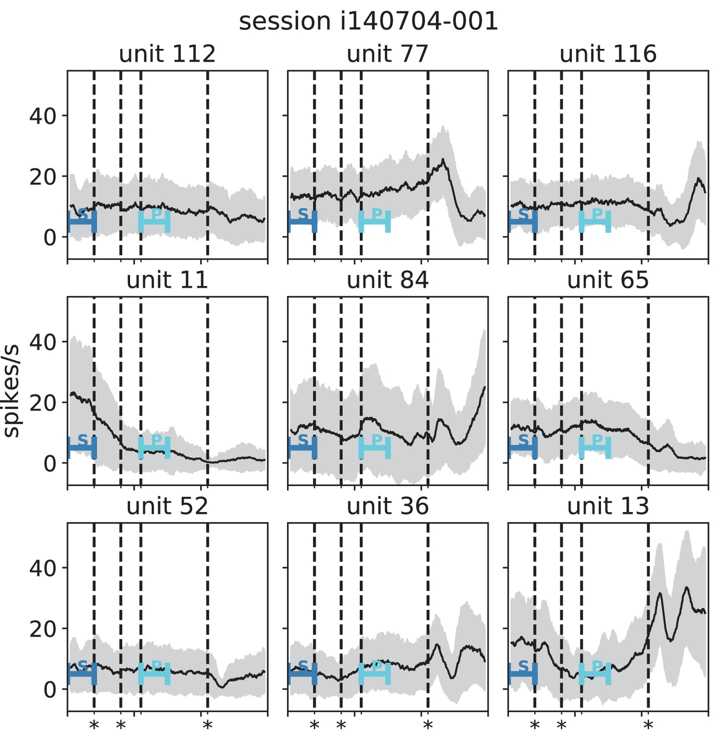
Stationarity of single-unit activity during a reach-to-grasp trial (monkey N, session i140704-001).

Analogous to Appendix 1—figure 5.

Appendix 1—figure 7

Download asset Open asset

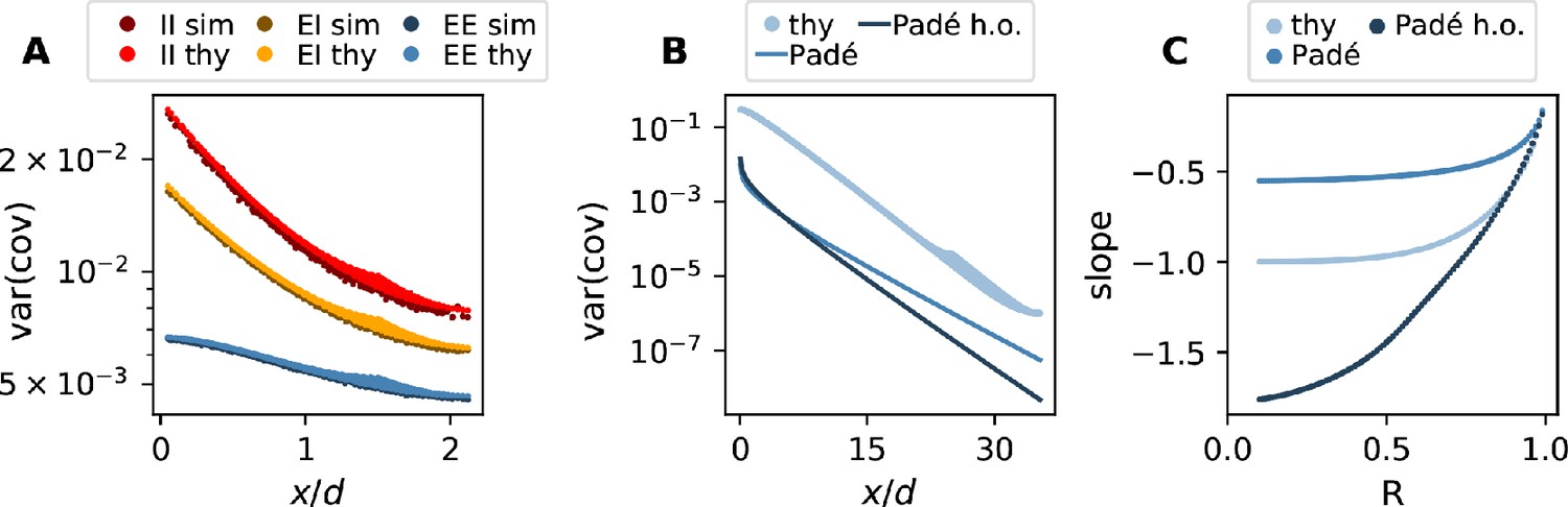
Comparison of simulation and theory.

(A) Variance of EE, EI, and II covariances as a function of distance. Darker dots are the results of the simulation. Lighter ones are the prediction of the discrete theory. (B) Variance of EE covariances as a function of distance (Equation (56) for variances). The lightest blue dots are the predictions of the discrete theory ( $μ_{a}$ replaced by the discrete Fourier transform of Equation (52), taking into account Section 7), the medium blue line is the (0,2)-Padé prediction ( $μ_{a}$ replaced by its Padé approximation Equation (53), taking into account Section 7), and the dark blue line is the higher order (1,2)-DLog-Padé prediction ( $μ_{a}$ replaced by its Padé approximation Equation (53), using Equation (57), and taking into account Section 7). (C) Fitted slope of linear regions in panel B for different spectral bounds $R$ (light blue: discrete theory, medium blue: Padé approximation, dark blue: higher order Padé approximation).

Tables

Appendix 1—table 1

Summary of exponential fits to distance-resolved variance of covariance.

For each value of E/I separation consistency $c$ the numbers of sorted putative neurons and the percentages of unclassified units, and therefore not considered for fitting SUs, are listed per resting state session, along with the resulting fits (Figure 4 in the main text)

C		E1	E2	N1	N2
0.6 (default)	#exc/#inh	56/50	67/56	76/45	78/62
	unclassified	0.078	0.075	0.069	0.091
	relative error	1.1157	1.0055	1.0097	1.0049
	1-slope fit	1.674	1.029	1.676	4.273
	I-I	1.919	0.996	1.647	4.156
	I-E	0.537	1.206	2.738	96100.688
	E-E	1.642	1.308	80308.482	94096.871
0.75	#exc/#inh	45/42	47/48	70/36	74/48
	unclassified	0.24	0.28	0.18	0.21
	relative error	1.1778	1.0141	1.0102	1.0090
	1-slope fit	1.357	0.874	1.420	2.587
	I-I	1.794	0.809	1.394	2.550
	I-E	0.496	1.123	3.682	40.852
	E-E	1.390	1.199	80548.500	10310.780

Appendix 1—table 2

Numbers of trials and single units per reach-to-grasp recording session.

Session names starting with “e” correspond to monkey E and session names starting with “i” to monkey N.

Session	N_trials	N_{single units}
e161212-002	108	129
e61214-001	99	118
e161222-002	102	118
e170105-002	101	116
e170106-001	100	113
i140613-001	93	137
i140617-001	129	155
i140627-001	138	145
i140702-001	157	134
i140703-001	142	142
i140704-001	141	124
i140721-002	160	96
i140725-002	151	106

Appendix 1—table 3

Parameters used to create theory figures. Decay constants in units of lattice constant $a$ .

	Figure 3B, C	Figure 3D, E	App 1—fig 7A	App 1—fig 7B
$N_{x}$	61	201	61	1,001	Number of neurons in x-direction
$N_{y}$	61	201	61	1,001	Number of neurons in y-direction
$q$	4	4	4	4	Ratio of excitatory to inhibitory neurons
$K_{E}$	100	100	100	100	Number of excitatory inputs per neuron
$K_{I}$	50	50	50	50	Number of inhibitory inputs per neuron
$d_{E}$	20	20	20	20	Decay constant of excitatory connectivity profile
$d_{I}$	10	10	10	10	Decay constant of inhibitory connectivity profile
$D$	1	1	1	1	Squared noise amplitude
$R$	0.95	0.95	0.8	0.95	Spectral bound
	exponential	exponential	exponential	exponential	Connectivity kernel

Appendix 1—table 4

Parameters used for NEST simulation and subsequent analysis.

Network parameters
$N$	2000	Number of neurons
$p$	0.1	Connection probability
$τ$	$1 ms$	Time constant
$σ_{μ}$	$1 Hz$	Standard deviation of external input
$σ_{noise}$	$0.1 Hz$	Standard deviation of noise
$R$	$[0.1, 0.2, \dots, 0.9]$	Spectral bound
$ϵ$	0.1	Parameter controlling difference of two network simulations
Simulation Parameters
$d t$	$0.1 ms$	Simulation step size
t_init	$100 ms$	Initialization time
t_sim	$2000000 ms$	Simulation time without initialization time
t_sample	$1 ms$	Sample resolution at which rates where recorded
Analysis Parameters
$N_{sample}$	200	Sample size
$T$	$100 ms$	Correlation time window