Figures and data in Separable neural signatures of confidence during perceptual decisions

Figures
Tables
Additional files

13 figures, 2 tables and 1 additional file

Figures

Figure 1

Download asset Open asset

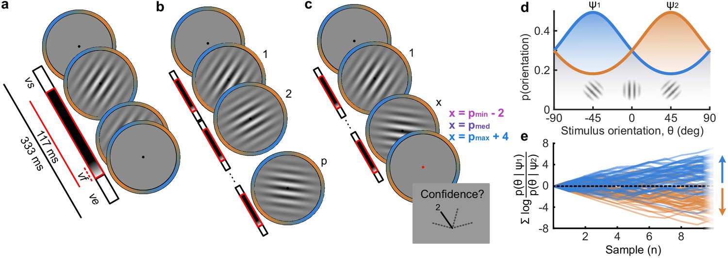
Procedure.

(a) Stimulus presentation: stimuli were presented at an average rate of 3 Hz, but with variable onset and offset ( $v s \in [83, 133]$ ms, ${v s}_{s} + {v e}_{s - 1} \geq 216$ ms; see Materials and methods). Stimuli were presented within a circular annulus which acted as a colour guide for the category distributions. The colour guide and the fixation point were present throughout the trial. (b) Free task: on each trial observers were presented with a sequence of oriented Gabors, which continued until the observer entered their response (or 40 samples were shown). 100 sequences were predefined and repeated three times. (c) Replay task: The observer was presented with a specific number of samples and could only enter their response after the cue (fixation changing to red). The number of samples (x) was determined relative to the number the observer chose to respond to on that same sequence in the Free task (p). There were three intermixed conditions, Less (x = *p_min* – 2; where *p_min* is the minimum p of the three repeats), Same (x = *p_med*; where *p_med* is the median p) and More (x = *p_max* + 4; where *p_max* is the maximum p of the three repeats of that predefined sequence). (d) Categories were defined by circular Gaussian distributions over the orientations, with means -45° ( $ψ_{1}$ , blue) and 45° ( $ψ_{2}$ , orange), and concentration $κ = 0.5$ . The distributions overlapped such that an orientation of 45° was most likely drawn from the orange distribution but could also be drawn from the blue distribution with lower likelihood. (e) The optimal observer accumulates the difference in the evidence for each category, which is defined as the log probability of the sample orientation ( $θ$ ) given the distributions. The perceptual decision is determined by the sign of the accumulated evidence, where the evidence accumulated across more samples better differentiates the true categories (example evidence traces are coloured by the true category).

Figure 2

Download asset Open asset

Behaviour and computational modelling.

(a) Proportion correct in each condition of the Replay task, relative to the Free task (orange horizontal lines). Individual data are shown in scattered points, error bars show 95% between- (thin) and 95% within- (thick) subject confidence intervals. Open red markers show the model prediction. (b) Distributions of the number of samples per trial in the Free task, and Replay task conditions (over all observers). (c) Difference in log-likelihood of the models utilising a covert bound relative to the models with no covert bound. On the left, the model fitting perceptual decisions only. The middle bar shows the difference in log-likelihood of the fit to confidence ratings with identical perceptual and confidence bounds. The right bar shows the difference in log-likelihood of the fit to confidence ratings of the model with an independent bound for confidence evidence accumulation. Error bars show 95% between-subject confidence intervals. (d) The computational architecture of perceptual and confidence decisions, based on model comparison. Perceptual and confidence decisions accumulate the same noisy perceptual evidence, but confidence is affected by additional noise ( $ε_{c}$ ) and a separate temporal bias ( $α_{c}$ ). This partial dissociation allows confidence evidence accumulation to continue after the observer has committed to a perceptual decision. (e) Predicted proportion correct compared to actual proportion correct for each observer, based on the fitted model parameters of the final computational model. The left panel shows proportion correct split by condition, and the right, split by confidence rating. (f) Regression coefficients from the GLM analysis showing the relationship between the optimal evidence L, and observers’ perceptual (top) and confidence (bottom) responses for trials split by condition. The right set of bars show the same analysis but with evidence accumulated up to four samples from the response cue.

Figure 3

Download asset Open asset

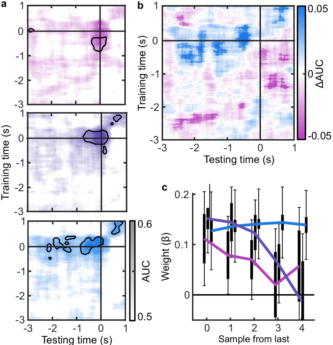
EEG signatures of premature perceptual decisions.

(a). Classifier AUC training at each time-point in the Free task and testing across time in the Less (top), Same (middle), and More (bottom) conditions of the Replay task. Black contours encircle regions where the mean is 3.1 standard deviations from chance (0.5; 99% confidence). (b) Difference in AUC between the More and Less conditions. Cluster corrected significant differences are highlighted. (c) The relationship between the evidence accumulated up to n samples prior to the response cue and the strength of the neural signature of response execution in each condition. Error bars show 95% within- (thick) and between-subject (thin) confidence intervals.

Figure 4

Download asset Open asset

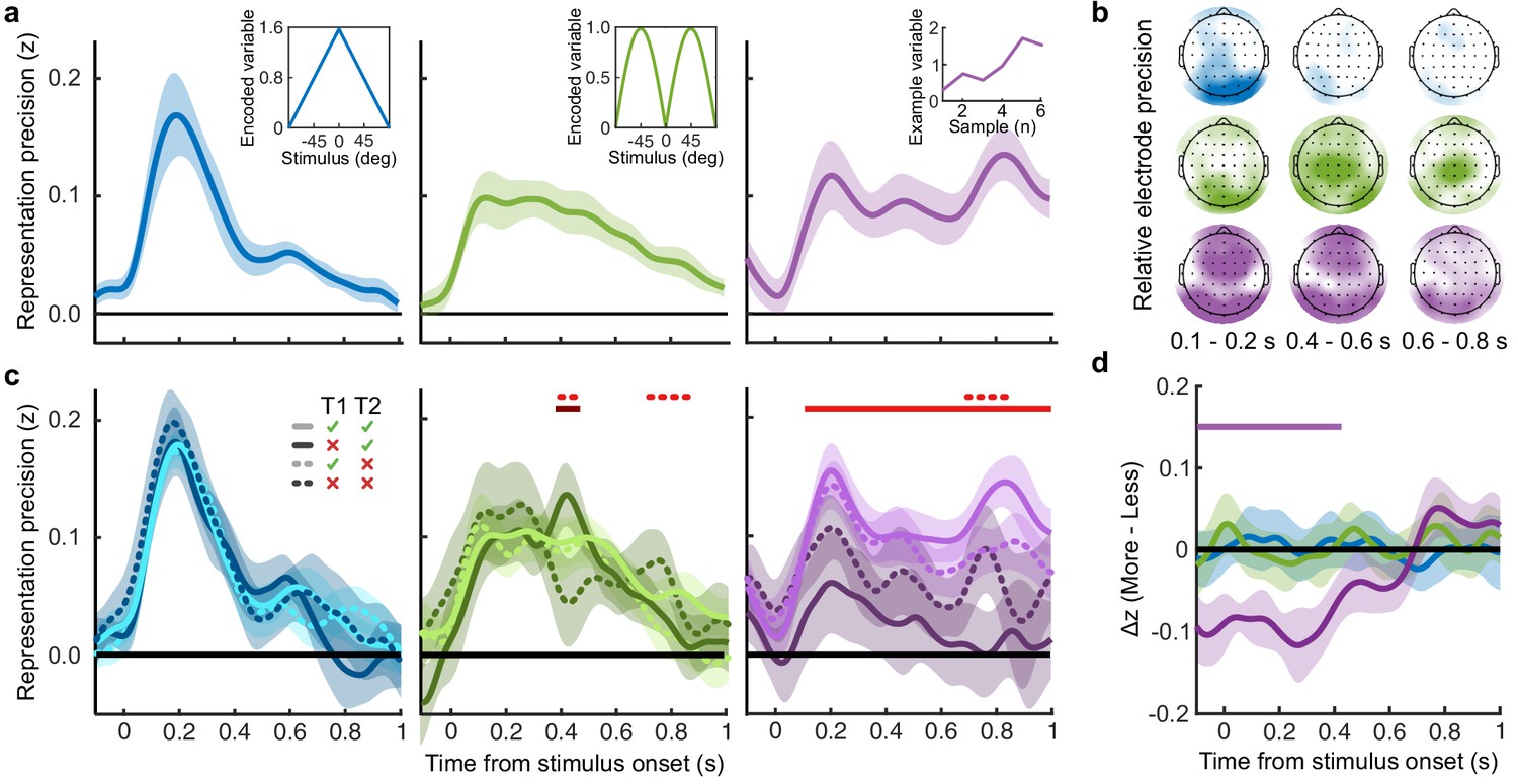
Representation of decision variables.

(a) Representation precision (Fischer transformed correlation coefficient, z) of stimulus orientation (blue, left), momentary decision update (green, middle), and accumulated decision evidence (purple, right). The encoded variables are shown in the insets (the accumulated evidence is the cumulative sum of the momentary evidence signed by the response, only one example sequence is shown). Shaded regions show 95% between-subject confidence intervals. (b) Relative electrode representation precision over three characteristic time windows (100–200 ms, left; 400–600 ms, middle; and 600–800 ms, right). (c) Representation precision for epochs leading to optimal and suboptimal perceptual (T1) and confidence (T2) responses. Lighter lines show perceptual decisions that match the optimal response, dashed lines show suboptimal confidence ratings. Dashed red horizontal lines show significant interactions between perceptual and confidence suboptimality. The light red horizontal line shows the significant effect of suboptimal perception and the dark red horizontal line shows the significant effect of suboptimal confidence. Shaded regions show 95% within-subject confidence intervals. (d) Difference in decoding precision between the More and the Less conditions for epochs corresponding to the last four samples of the trial. The purple horizontal line shows the significant difference in decoding of accumulated evidence.

Figure 5

Download asset Open asset

Clusters of behaviourally relevant representations and their sources.

(a) Log likelihood ratio (LLR) of the data given the hypothesis that decoding precision varies with behavioural suboptimalities, against the null hypothesis that decoding precision varies only with measurement noise. Perceptual (Type-I) behaviour is shown on top and confidence (Type-II) behaviour is shown on the bottom. Clusters where the log posterior odds ratio outweighed the prior are circled, only the bold area of the perceptual cluster was further analysed. Time series (left) show the maximum LLR of electrodes laterally, with frontal polar electrodes at the top descending to occipital electrodes at the bottom. Scalp maps (right) show the summed LLR over the indicated time windows. (b) Left: representation precision (z) training and testing on signals within the clusters. Colours correspond to the circles in (a), with the dark green bar showing the combined decoding precision of the anterior and posterior confidence clusters, and the black bar showing the combined representation precision of all clusters. Right: Representation precision of the last four samples in the Less and the More conditions for the combined confidence representation and the perceptual representation. Error bars show 95% within-subject confidence intervals. (c) ROIs (defined by mindBoggle coordinates; Klein et al., 2017): lateral occipital cortex (blue); superior parietal cortex (green); orbitofrontal cortex (orange); and rostral middle frontal cortex (red). (d) ROI time series for Noise Max (black) and Noise Min (coloured) epochs, taking the average rectified normalised current density (z) across participants. Shaded regions show 95% within-subject confidence intervals, red horizontal lines indicate cluster corrected significant differences. Standardised within-subject differences are traced above the x-axis, with the shaded region marking z = 0 to z = 1.96 (95% confidence). (e) Standardised regression weight (t-statistic) of the GLM comparing observers’ confidence ratings to those predicted from the activity localised to the orbitofrontal cortex. The shaded region shows the 95% between-subject confidence interval, and the red horizontal line marks the time-window showing cluster-corrected significant differences from 0.

Appendix 1—figure 1

Download asset Open asset

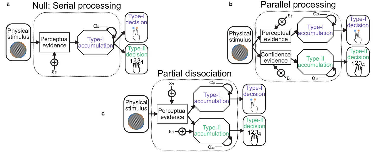
Schematic of possible relationships between perceptual (Type-I) and confidence (Type-II) evidence accumulation.

(a) Same evidence accumulation processes: Type-I (perceptual) and Type-II (confidence) decisions are different responses to the same evidence: each sample of perceptual evidence is disrupted by a sample of sensory noise ( $ε_{s}$ ) drawn from a zero-mean Gaussian with standard deviation $σ$ , and accumulated with a temporal bias described by $α_{s}$ . (b) Parallel processing: Type-I and Type-II decisions rely on entirely separate processing of the same physical stimulus: the confidence decision also incurs noise and temporal integration bias (with subscript c), but these may vary independently of the perceptual processing suboptimalities (subscript s). (c) Partial dissociation: Type-I and Type-II decisions rely on partially dissociable accumulation of the same evidence.

Appendix 2—figure 1

Download asset Open asset

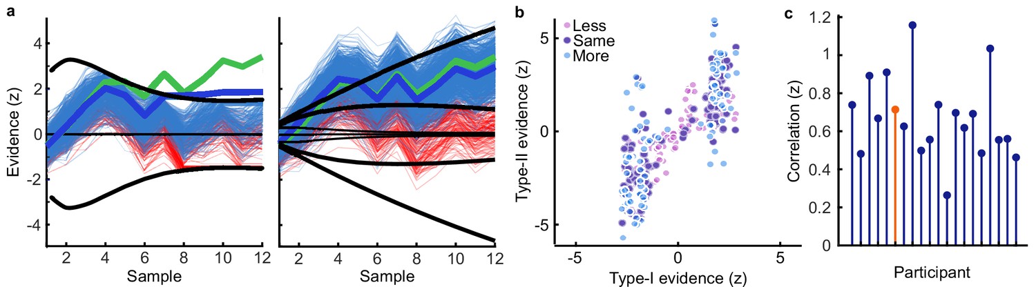
Model simulation of accumulated evidence for perceptual and confidence decisions.

(a) Example trial from one observer showing simulated evidence traces agreeing with the observer’s response (blue) and a sample of example traces which did not agree (red). The perceptual decision is shown on the left. An evidence trace was taken to agree with the observer’s decision if the corresponding bound was reached prior to the opposing bound, or if no bound was reached but the final accumulated evidence was in favour of the chosen option. The median evidence trace (thick blue line) was calculated assuming the evidence that reached the bound early was maintained until the response was entered. For the confidence rating (right) we compared the median evidence from traces where the final accumulator (plus one additional sample of noise) agreed with the observer’s confidence rating. We examined the difference from the ideal accumulated evidence (thick green line) relative to the likelihood of the observers’ rating given all simulated evidence traces. (b) Median final simulated accumulated evidence for the perceptual decision (abscissa), and the confidence decision (ordinate) for all trials of the example observer, colours indicate the condition. (c) Correlation (Fisher transformed z) between perceptual and confidence evidence for each observer. The example observer is highlighted in orange.

Appendix 3—figure 1

Download asset Open asset

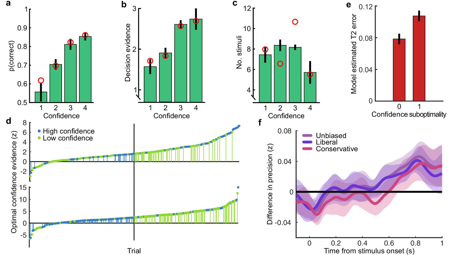
Confidence behaviour.

(a) proportion correct (in the perceptual decision) by confidence rating. (b) Decision evidence (based on the presented samples) by confidence rating. (c) Number of samples presented by confidence rating. In all plots, error bars show 95% within-subject confidence intervals. Red circles show the predictions of the best fitting confidence model (Appendix 1). (d) Confidence responses of two observers (top and bottom panels) on all trials sorted by the confidence evidence of the optimal observer. The median confidence evidence (shown by a black vertical line) defines an optimal confidence observer whose confidence above this median are rated high. Observers’ high confidence ratings are shown in blue and low confidence ratings in green. Suboptimal confidence ratings, where human and optimal confidence observers do not match, are indicated with small vertical segments (green for Type-II misses and blue for Type-II false alarms). Negative confidence evidence corresponds to incorrect perceptual decisions. The observer shown on top clearly has fewer suboptimal responses compared with the observer below, and the frequency of suboptimal responses decreases further from the median. (e) Model estimated confidence error by confidence rating suboptimality (0 = the observer’s confidence rating was the same as the optimal observer, 1 = suboptimal confidence rating). (f) The effect of response bias on the analysis of suboptimal confidence in the EEG representation of accumulated evidence. Observers’ confidence ratings were compared to an unbiased optimal observer (purple), and two biased (but otherwise optimal) observers, who respond with high confidence on 35% and 65% of trials (making the human observers relatively more liberal and conservative with their response strategy in comparison). Thick lines show the within-subject difference in precision (Fisher transformed correlation) between trials where the human observers’ confidence ratings correspond to the (un/biased) optimal observer and suboptimal confidence ratings. Shaded regions show the 95% between-subject confidence intervals on the difference.

Appendix 4—figure 1

Download asset Open asset

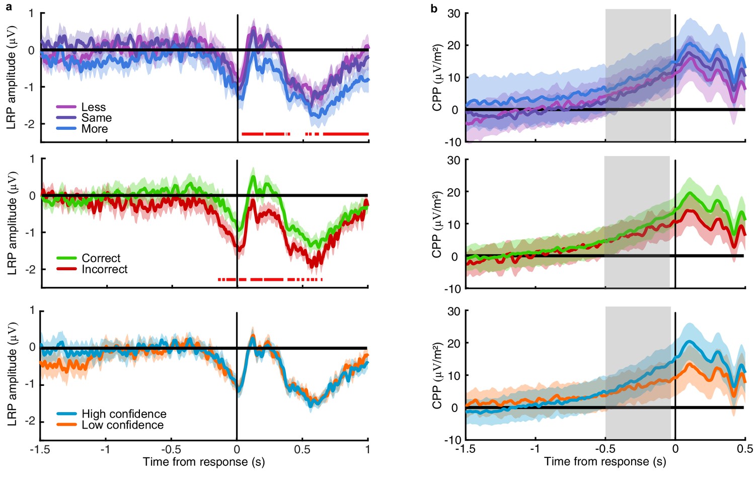
Amplitude modulations with task variables.

(a) The Laterised readiness potential by condition (top), perceptual decision accuracy (middle) and reported confidence (bottom). Horizontal red lines mark significant differences in amplitude. (b) Central Parietal Positivity, with the same comparisons. Shaded regions show 95% within subject confidence intervals, and the region of slope comparison for the CPP is highlighted in grey.

Appendix 5—figure 1

Download asset Open asset

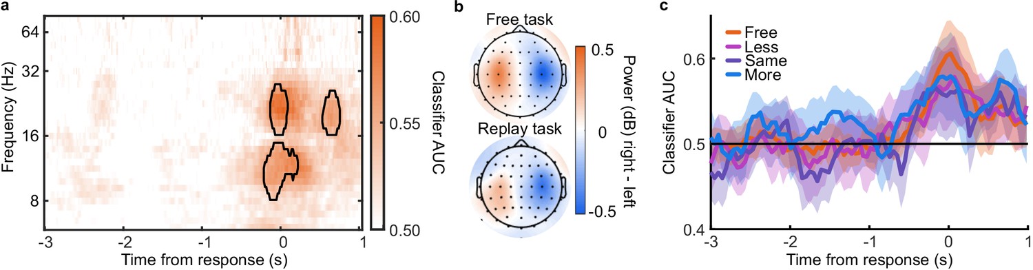
Response Classification analysis.

(a) Classifier AUC training and testing at each time point (abscissa) based on the power (dB) in each frequency band (ordinate). Clusters where average performance is greater than 3.1 standard deviations (99% confidence) from baseline (0.5) are circled in black. (b) Scalp map of the difference in power for right- compared to left-handed responses averaged over 8 to 32 Hz and −0.5 to 05 s around the response. (c) Classifier performance (AUC) training and testing at each time point, in each condition of the Replay task and in the Free task.

Appendix 6—figure 1

Download asset Open asset

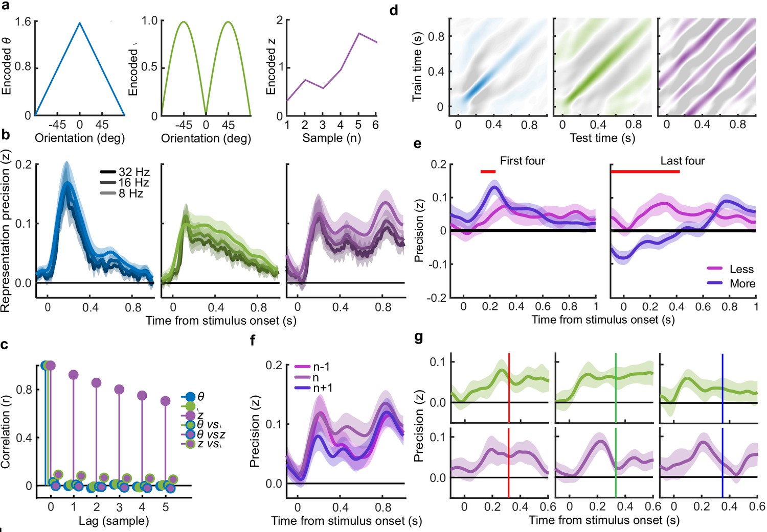
Encoding variable regression.

(a) Encoded variables used to regress EEG signals. The encoded orientation ( $C_{θ}$ , left) and encoded momentary decision update ( $C_{l}$ , middle) were dependent on the orientation presented to the observer. The encoded accumulated evidence ( $C_{z}$ ) varied over all presented orientations in a trial, the figure on the right shows only one example. (b) Representation precision of encoding variables using different low-pass filters. (c) Cross correlation between encoding variables over consecutive samples. (d) Temporal generalisation of representations: the regression weights were calculated on EEG signals at each time point and precision was tested across time. Colour scales are relative to the maximal precision, with zero precision in white and negative in grey (a sign flip of the regression weights). (e) Representation precision of the accumulated evidence for the first (left) and last (right) four stimuli of the Less and More conditions. Shaded error bars show the 95% within subject confidence intervals, red horizontal bars mark cluster corrected significant differences between conditions. (f) Representation precision of the previous (n-1), current (n) and future (n+1) accumulated evidence, based on the EEG signals locked to the current epoch. (g) Representation precision of the momentary decision update (top) and the accumulated evidence (bottom) for epochs separated by the timing of the subsequent stimulus, shown in coloured bars (317 ms, red, left; 333 ms, green, middle; and 350 ms blue, right).

Appendix 8—figure 1

Download asset Open asset

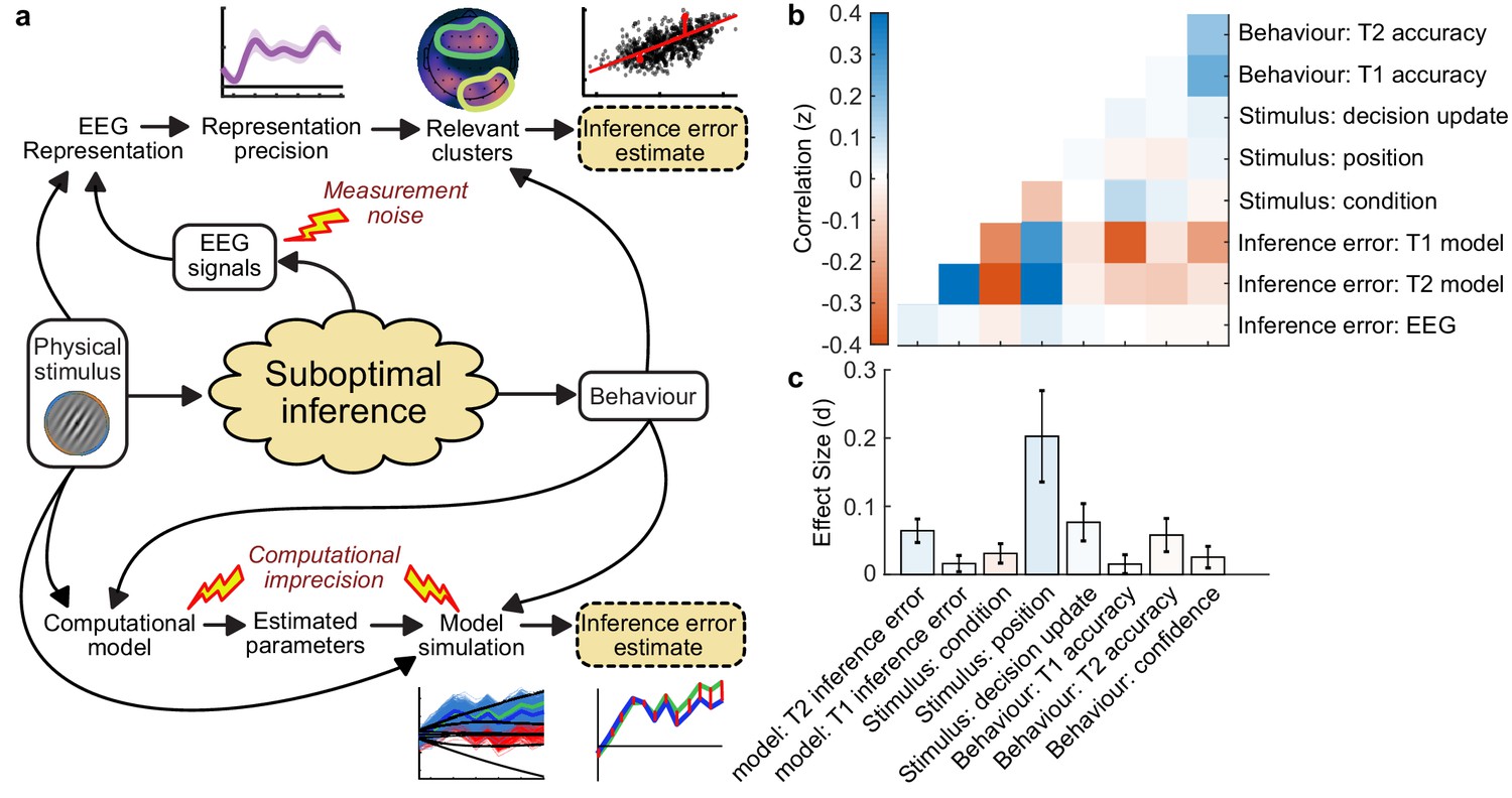
Estimating inference error.

(a) Two approaches to estimate inference error. It is assumed the observer’s behaviour is based on a suboptimal inference over the physical stimulus. We do not have access to the single-sample inference error, but can estimate it using the measured variables: the physical stimulus properties, the behaviour, and the EEG signals. Two approaches are outlined: The EEG inference error estimate, which relies on the error of the representation of the accumulated evidence, in clusters where the precision of the representation is related to suboptimal behaviour; and the model error, which relies on simulating the processing of the evidence based on the fitted model parameters, and taking the median of simulated traces which concur with the observer’s response. (b) Correlation between variables measured from behaviour, the stimulus input, and the estimated inference error. (c) Effect size on the difference between Noise Min and Noise Max epochs.

Appendix 9—figure 1

Download asset Open asset

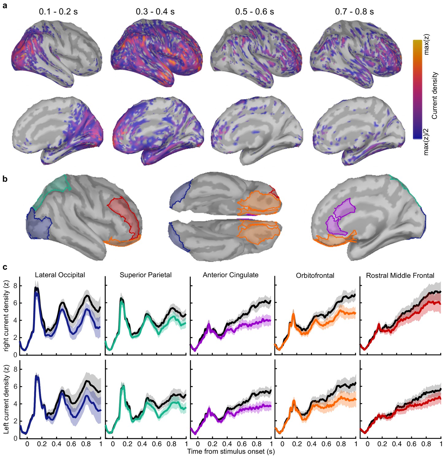
Regions of interest and corresponding current density.

(a) Average rectified normalised current density in Noise Min epochs for the corresponding time windows, filtered above the half-maximum amplitude (b) Regions of interest based on Mindboggle coordinates. (c) Average normalised rectified current density in the right (top) and left (bottom) hemispheres. Noise Min epochs are shown coloured, Noise Max in black, with shaded regions showing the 95% within-subject confidence interval.

Tables

Appendix 1—table 1

Average parameter values.

Table shows the average values and the sum of BIC across participants. The large difference in the average log-likelihood (LLH) across tasks is due to the fact the Free task model was fit to both when and what observers responded, whereas in the Replay task only the response was fit. Red values show the fixed parameters.

Free task
Model	$σ$	$α$	c	$μ_{U}$	$σ_{U}^{2}$	a	b	$λ$	l	LLH	∑BIC
Full	0.83	0.98	−0.04	425	0.52	0.10	6.04	1.93	0.016	−734.91	30423.01
$α = 1$	0.83	1.00	0.00	430	0.50	0.13	6.61	2.03	0.014	−734.97	30311.59
c = 0	0.80	0.92	0.00	452	0.54	0.11	5.28	2.01	0.017	−736.86	30387.02
$μ_{U} = 400$	0.76	0.94	0.00	400	0.52	0.09	5.52	2.23	0.016	−739.77	30503.40
$σ_{U}^{2} = 1$	0.69	0.96	−0.02	435	1.00	0.10	6.34	1.97	0.015	−754.18	31079.84
a = 0.1	0.77	0.92	0.03	417	0.52	0.10	5.78	2.20	0.016	−735.48	30331.75
b = 5.5	0.78	0.94	0.02	410	0.64	0.13	5.50	1.79	0.013	−742.18	30599.67
l = 0.001	0.82	0.98	0.01	400	0.48	0.10	4.77	2.22	0.001	−730.66	30139.17
c = 0; l = 0.001	0.79	0.94	0.00	397	0.51	0.10	4.52	2.26	0.001	−732.66	30104.74
c = 0; l = 0.001; a = 0.1	0.77	0.94	0.00	403	0.52	0.10	5.37	2.13	0.001	−742.42	30381.13
Replay Task - no-bound
Model	$σ$	$α$	c	$μ_{U}$	$σ_{U}^{2}$	a	b	$λ$	l	LLH	∑BIC
Full	0.47	0.90	0.05	~	~	~	~	~	0.012	−81.13	3701.44
$α = 1$	0.56	1.00	0.10	~	~	~	~	~	0.012	−92.21	4030.55
c = 0	0.48	0.90	0.00	~	~	~	~	~	0.009	−82.73	3651.38
l = 0.001	0.50	0.91	0.06	~	~	~	~	~	0.001	−82.05	3624.39
c = 0; l = 0.001	0.51	0.90	0.00	~	~	~	~	~	0.001	−83.64	3573.67
Replay task - bound
Model	$σ$	$α$	c	$μ_{U}$	$σ_{U}^{2}$	a	b	$λ$	l	LLH	∑BIC
Full	0.44	0.87	0.10	~	~	0.17	8.68	11.71	0.012	−79.81	3991.09
c = 0; l = 0.001	0.48	0.88	0.00	~	~	0.13	8.58	15.55	0.001	−82.22	3859.24
c = 0; l = 0.001; a = 0.1	0.48	0.88	0.00			0.10	8.91	15.88	0.001	−82.38	3751.55

Appendix 1—table 2

Average parameter values for perceptual and confidence behaviour.

Bound parameters with subscript c describe the criteria for confidence ratings, which take the same form as the perceptual decision bound. They have the same minimum and scale, but different rates of decline, such that $λ$ _c1determines the upper bound on a confidence rating of 1, and the lower bound on a rating of 2. Apart from the ‘Serial’ and ‘Serial continued’ models, parameters for perceptual decisions were fixed to those fit in the winning perceptual decision model and the listed parameters affect only the confidence evidence accumulation.

Model	$σ$	$α$	a	b	$λ$	a_c	b_c	$λ$ _c1	$λ$ _c2	$λ$ _c3	LLH	∑BIC
Serial	0.73	0.92	0.10	12.74	17.07	0.07	0.64	1.28	6.81	31.38	−428.36	18275.28
Serial continued	0.67	0.91	0.13	9.60	17.98	0.06	0.53	0.66	7.08	30.41	−424.88	18135.83
Parallel	0.76	0.90	~	~	~	0.01	0.58	0.18	7.51	30.68	−437.25	18288.50
Partial - same sigma	0.00	0.89	~	~	~	0.06	0.47	1.03	6.77	25.92	−446.41	18540.68
Partial - accumulation noise	0.45	0.91	~	~	~	0.03	0.58	0.50	7.71	31.03	−421.59	17662.25
Partial - read-out noise	0.12	0.90	~	~	~	0.02	0.52	1.85	8.63	37.39	−417.94	17516.29
Partial - same alpha	0.12	0.88	~	~	~	0.02	0.52	0.98	8.22	35.16	−423.02	17605.29