Novel neuroanatomical integration and scaling define avian brain shape evolution and development
Figures
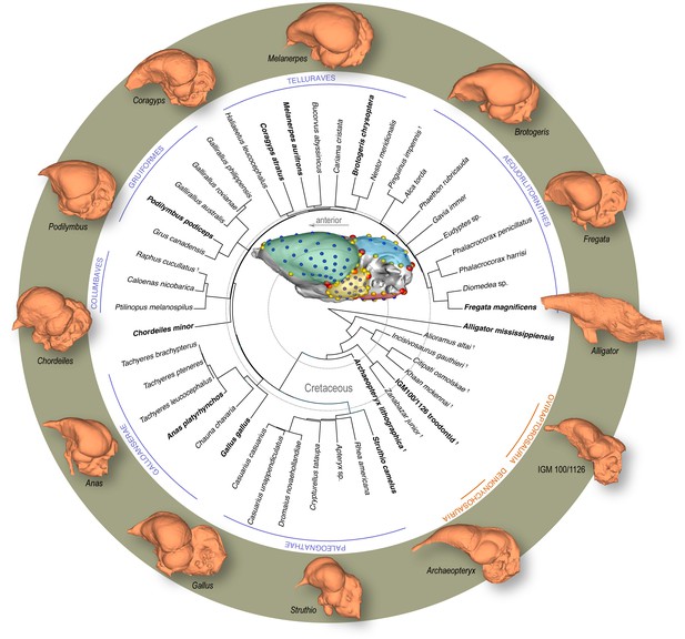
Time-calibrated phylogeny of avialan and non-avialan coelurosaurs sampled in this study, with Alligator mississippiensis as outgroup.
Center image shows discrete (red), curve (yellow), and surface (blue) landmarks used to characterize endocranial shape including the cerebrum (green), optic lobe (yellow), cerebellum (blue), and medulla (red). Lateral views of select endocranial models, indicated by bolded taxonomic names on the phylogeny, highlight the neuroanatomical variation observed across taxa. See Supplementary file 1a for list of specimens sampled for the interspecific dataset and Supplementary file 1b for the landmark scheme used in this study.
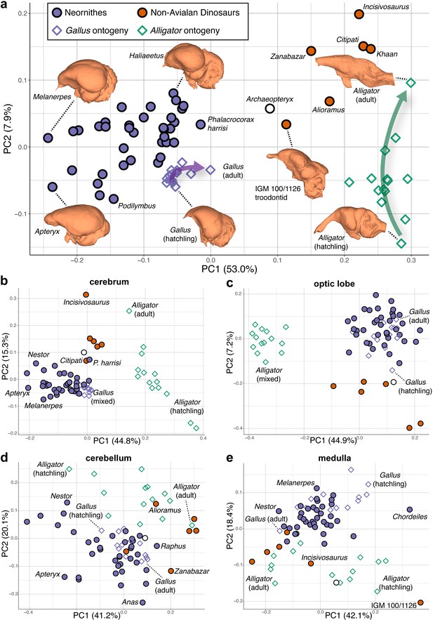
Morphospaces constructed from first two principal components (PC) of neuroanatomical shapes.
These plots illustrate the distribution of shape variation in the (a) overall endocranial shape, where the arrows denote postnatal developmental trajectories of Alligator (green) and Gallus (purple); (b) cerebrum; (c) optic lobe; (d) cerebellum; and (e) medulla. Regional shape data are locally aligned. See text for details. The following figure supplement is available for Figure 2—figure supplement 1. PC morphospaces with full specimen labels.
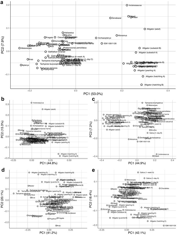
Morphospaces constructed from first two principal components of neuroanatomical shape.
These plots illustrate the distribution of shape variation in the (a) overall endocranial shape; (b) cerebrum; (c) optic lobe; (d) cerebellum; and (e) medulla. Regional shape data are locally aligned.
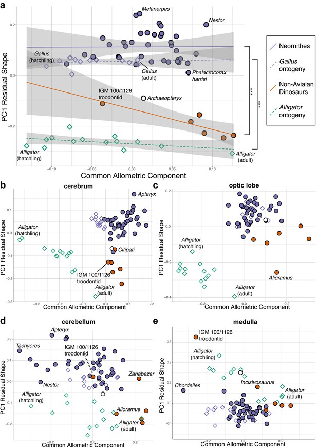
Bivariate plots of PC1 of residuals from the common allometric component (CAC) against scores along CAC (Mitteroecker et al., 2004).
These plots illustrate neuroanatomical deviations from the overall shape-to-size allometric trend in the (a) endocasts (band indicates 95% confidence band), where the null hypothesis that the allometric trajectories between Neornithes and non-avialan dinosaurs and between Alligator and Gallus are the same is rejected statistically (*** denotes p<0.001); (b) cerebrum; (c) optic lobe; (d) cerebellum; and (e) medulla. For each subregion, locally aligned shapes and regional log-transformed centroid sizes were used. See text for details. The following figure supplement is available for Figure 3—figure supplement 1. Principal components (PC) plots of PC1 of residuals from CAC against CAC with full specimen labels.
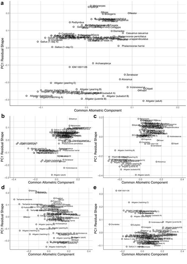
Bivariate plots of PC1 of residuals from the common allometric component (CAC) against scores along CAC.
These plots illustrate neuroanatomical deviations from the overall shape-to-size allometric trend in the (a) overall endocasts; (b) cerebrum; (c) optic lobe; (d) cerebellum; and (e) medulla. For each subregion, the locally aligned shape and regional centroid size were used.
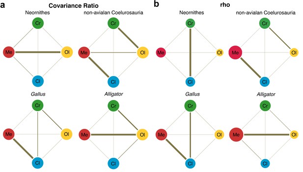
Pattern of correlation across locally aligned neuroanatomical shapes.
(a) Network diagrams based on between-region covariance ratios (CR) (Supplementary file 1d, f; Adams, 2016). (b) Network diagrams based on correlation coefficient, rho, from maximum likelihood analysis (Supplementary file 1d, f; Goswami and Finarelli, 2016), where the size of the circles represent the degree of within-region correlation. In both sets of diagrams, the thickness of the line segments between regions indicates relative strength of the correlation. Note that the line thickness is based on values within each analysis (i.e., not comparable between diagrams), where the cut-off point is the mean correlation value. Abbreviations: Cl, cerebellum; Cr, cerebrum; Ol, optic lobe; Me, medulla. See text for details. The following figure supplement is available for Figure 4—figure supplement 1. Network diagrams of integration within and between globally aligned neuroanatomical regions.
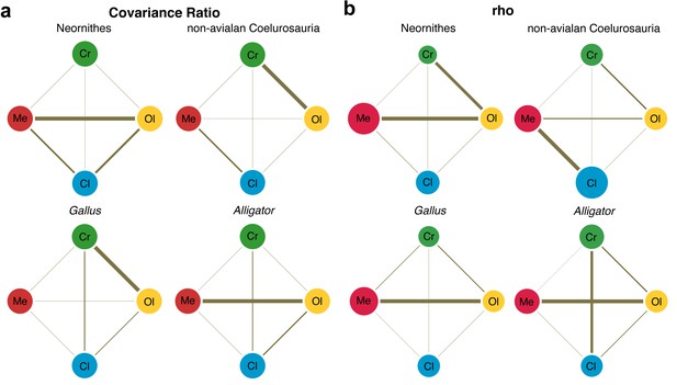
Pattern of correlation across globally aligned neuroanatomical shapes.
(a) Network diagrams based on between-region covariation ratios (CR) (Adams, 2016). (b) Network diagrams based on correlation coefficient, rho, from maximum likelihood analysis (Goswami and Finarelli, 2016), where the size of the circles represent the degree of within-region correlation. In both sets of diagrams, the thickness of the line segments between regions indicates relative strength of the correlation. Note that the line thickness is based on values within each analysis (i.e., not comparable between diagrams), where the cut-off point is the mean correlation value. Abbreviations: Cl, cerebellum; Cr, cerebrum; Ol, optic lobe; Me, medulla.
Additional files
-
Supplementary file 1
Supplementary tables related to this study.
(a) List of taxa sampled for this study, with the exclusion of Alligator and Gallus. Institutional abbreviations: AMNH, American Museum of Natural History, New York, NY, USA; BMNH, British Museum of Natural History, London, UK; FMNH, Field Museum of Natural History, Chicago, IL, USA; KU, University of Kansas, Lawrence, KS, USA; NMNH, National Museum of Natural History, Washington DC, USA; TCWC, Texas Cooperative Wildlife Collection, College Station, TX, USA; TMM, Texas Memorial Museum, Austin, TX, USA; WDC, Wyoming Dinosaur Center, Thermopolis, WY, USA. (b) List of discrete landmarks and density of semi-landmarks for each neuroanatomical region. (c) Phylogenetic signal (Blomberg’s K), allometry, and evolutionary allometry in endocranial shape. Results generated using physignal, procD.lm, procD.pgls functions in geomorph R package v3.2.1 (Adams and Otárola-Castillo, 2013). Results from analysis on globally and locally aligned regions are presented as first and second values within a cell, respectively. Allometry evaluated with log-transformed centroid size of the entire endocast and local region, respectively. *, **, and *** indicate p<0.05, <0.01, and <0.001, respectively, based on 1000 pseudo-replications. (d) Integration within and between locally aligned neuroanatomical regions. Degree of integration is measured by correlation coefficient from two-block partial least-squares analysis (RPLS; upper off-diagonal) and correlation coefficient (ρ; diagonal, lower off-diagonal) using the R packages geomorph v3.2.1 (Adams and Otárola-Castillo, 2013) and EMMLiv2 v0.0.3 (Goswami and Finarelli, 2016), respectively. Interspecific analyses are phylogenetically corrected using phylogenetic generalized least-squares method. (e) Integration within and among globally aligned neuroanatomical regions. The degree of integration is measured by correlation coefficient from two-block partial least-squares analysis (RPLS; upper off-diagonal) and correlation coefficient (ρ; diagonal, lower off-diagonal) using the R packages geomorph v3.2.1 (Adams and Otárola-Castillo, 2013) and EMMLi v2 v0.0.3 (Goswami and Finarelli, 2016), respectively. Interspecific analyses are phylogenetically corrected using phylogenetic generalized least-squares method. (f) Integration between neuroanatomical regions using covariance ratios (CR) (Adams, 2016). Degree of integration between globally aligned regional shapes are listed in the upper off-diagonal elements and that of locally aligned regional shapes in the lower off-diagonal elements. Interspecific analyses are phylogenetically corrected using phylogenetic generalized least-squares method. (g) Comparison of integration among neuroanatomical regions using the compare.pls function in the geomorph R package (Adams and Otárola-Castillo, 2013; Adams and Collyer, 2016). ‘+’ and ‘–’ denote greater and lesser integration in Neornithes and Gallus compared to non-avialan coelurosaurs and Alligator, respectively. Integration among species calculated upon phylogenetic correction. *, **, and *** indicate p<0.05, <0.01, and <0.001 (one-tailed), respectively, based on 1000 pseudo-replications. Numbers preceding and following ‘/’ indicate results based on globally and locally aligned data, respectively.
- https://cdn.elifesciences.org/articles/68809/elife-68809-supp1-v1.docx
-
Transparent reporting form
- https://cdn.elifesciences.org/articles/68809/elife-68809-transrepform-v1.pdf


