Locating macromolecular assemblies in cells by 2D template matching with cisTEM
- Howard Hughes Medical Institute, Janelia Research Campus, United States
- Howard Hughes Medical Institute, RNA Therapeutics Institute, The University of Massachusetts Medical School, United States
- Structural and Computational Biology Unit, European Molecular Biology Laboratory (EMBL), Germany
- Collaboration for joint PhD degree between EMBL and Heidelberg University, Faculty of Biosciences, Germany
Figures
Figure 1 with 1 supplement

cisTEM GUI implementation of 2DTM.
(a) Screenshot showing the results of a 2DTM search in the cisTEM GUI (located in the ‘Experimental’ tab). The panel on the left shows all images searched. Images may be searched individually (column #1) or as batch jobs (column #2). The Results tab shows the locations, orientations and SNR values of each detected target in a list, as well as the original image (b) (membrane highlighted in yellow), the maximum intensity projection (MIP, c) and the plotted result (d), which shows the best-matching orientation of the template at each detected location. The survival histogram (subpanel in (a)) shows the SNR values for all search locations (blue line) and compares this with the survival histogram of Gaussian noise (red line). This is used to establish the threshold at which a single false positive is expected per image. Scale bar in (b) = 500 Å.
Figure 1—figure supplement 1
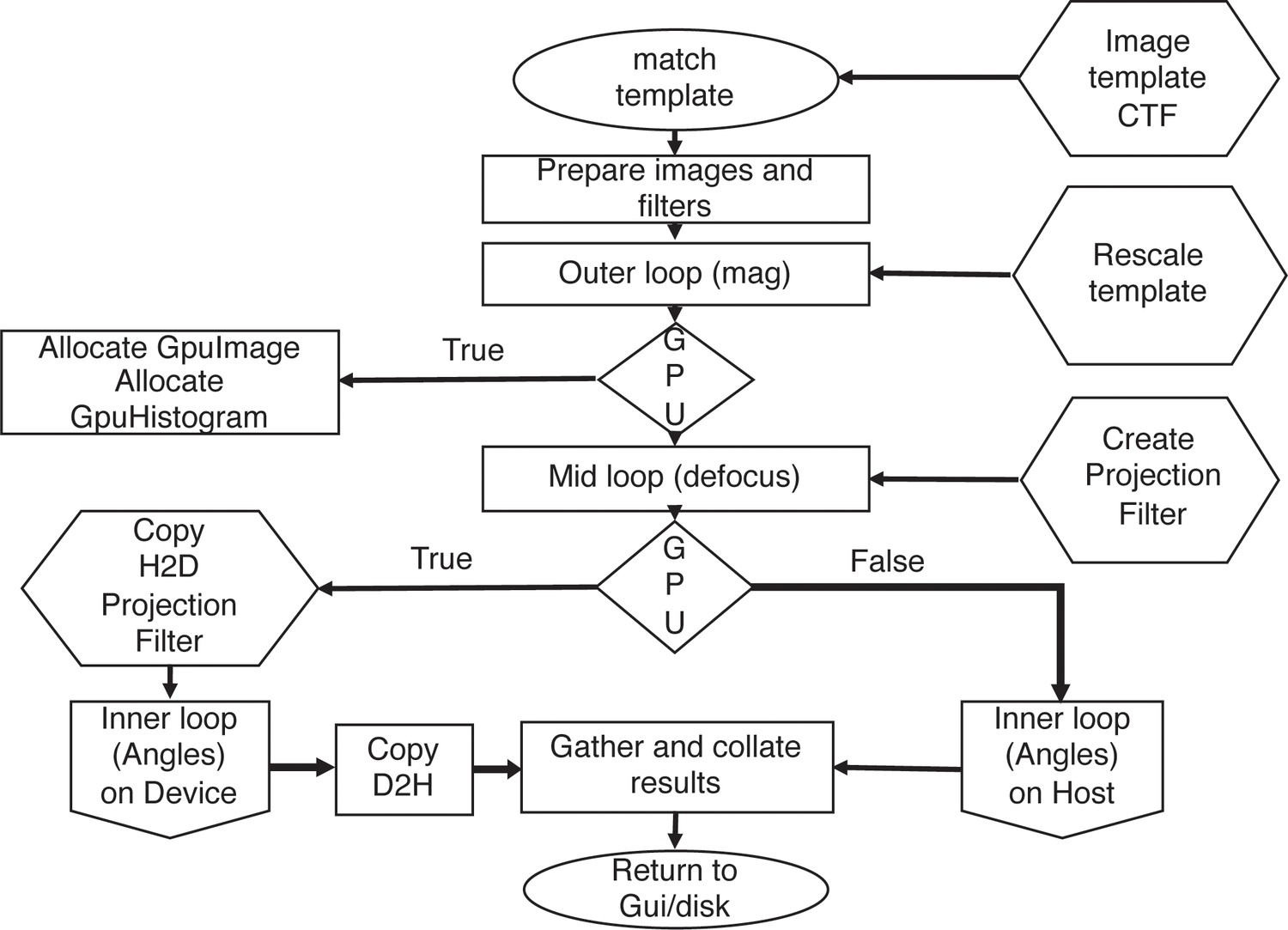
The 2DTM matching algorithm as implemented in cisTEM.
Inputs to various stages are in hexagons. If the GPU is used, all memory allocations are handled by the TemplateMatchingCore class via calls to the underlying GpuImage class. The whitening filter and CTF are combined on the host and if needed, copied to the GPU once for each defocus plane searched. The inner loop (Figure 2—figure supplement 1) is executed and results returned to the host.
Figure 2 with 1 supplement
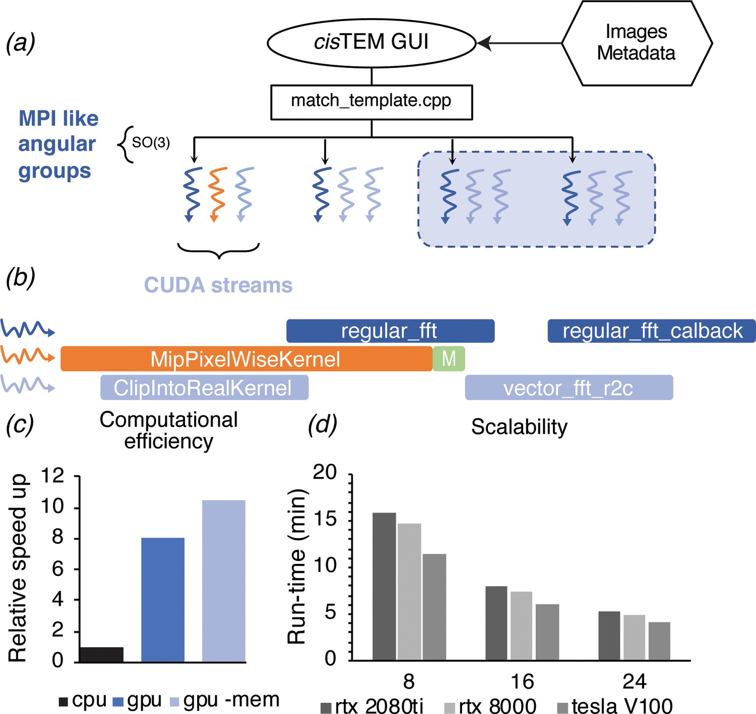
GPU acceleration of 2DTM in cisTEM.
(a) The angular search space is distributed among any number of processors using the home-grown MPI-like socket communication in the cisTEM GUI (Grant et al., 2018). Unlike MPI, if fewer processors are available than requested (shaded box) processing may still proceed. (b) To expose further parallelism, additional host threads may be requested to subdivide each angular group to maximize occupancy on the GPU. Each host thread queues up a series of GPU kernels into its respective stream, and then returns to calculate the next projection and initiates its transfer to the GPU (green box). This way, close to 100% of the CPU and GPU is used during computation. (c) GPU acceleration relative to optimized CPU-based calculation, of which 85% is spent on MKL-based FFTs. Kernel-fusion using cuFFT callbacks and custom data structures combined with flexible kernel launch parameters ensure the GPUs stay saturated, enabling an 8x speedup. A total of 10.5x speedup is achieved by optimizing data throughput using the vectorized FP16 format for storing results. (d) The code scales nearly linearly with the number of GPUs and tracks with the total memory bandwidth of a given model. All timings were obtained using a padded K3 image with 4096 × 5832 pixels, and searching one defocus plane with 2.5°/1.5° angular steps.
Figure 2—figure supplement 1
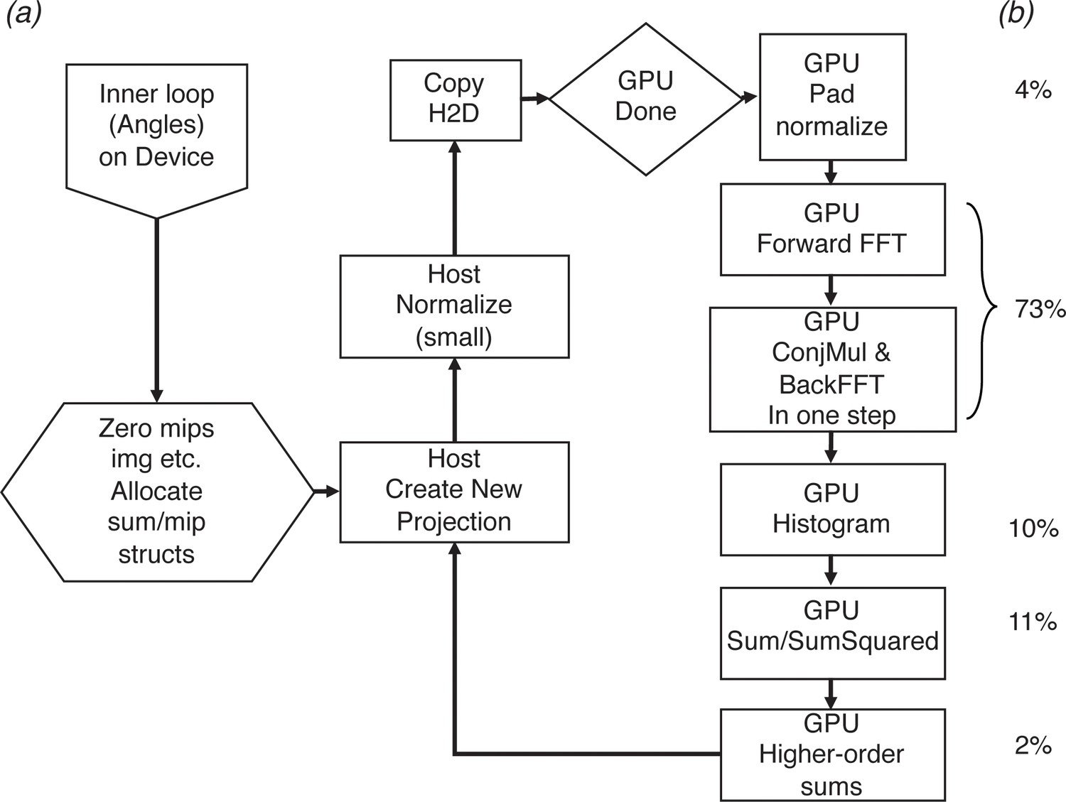
GPU implementation and runtime profiling.
(a) The 2DTM matching inner loop as implemented on the GPU in cisTEM. (b) Approximate percentage of run time for each step. The relative percentages can vary based on the automatic load balancing due to the combination of CUDA streams and mixed kernel launch configurations that restrain some low-complexity operations to a small subset of available streaming multi-processors via grid-stride loops.
Figure 3 with 1 supplement
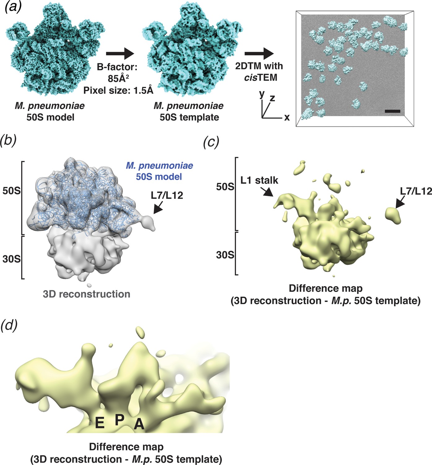
2DTM detects ribosomes in Mycoplasma pneumoniae cells.
(a) An overview of 2DTM: a cryoEM-like density was generated from an M. pneumoniae 50S model, a B-factor was applied and the resulting template used to identify locations and orientations of 50S in 2D images of M. pneumoniae cells with 2DTM implemented in cisTEM. Scale bar = 500 Å (b) 20 Å filtered 3D reconstruction generated using the locations and orientations of 5080 50S subunits detected in 220 images using 2DTM with a M. pneumoniae 50S template, showing clear density for the 30S ribosomal subunit (not included in the template). (c) Difference map showing the regions of the 3D reconstruction that differ from the 50S 2DTM search template. Arrows indicate additional density consistent with 70S ribosome structures. The difference map was generated with the same threshold as in (b). (d) A region of the difference map shown in (c), showing tRNAs in characteristic arrangements in the E, P, and A sites of the 30S subunit. M.p.: M. pneumoniae.
Figure 3—figure supplement 1
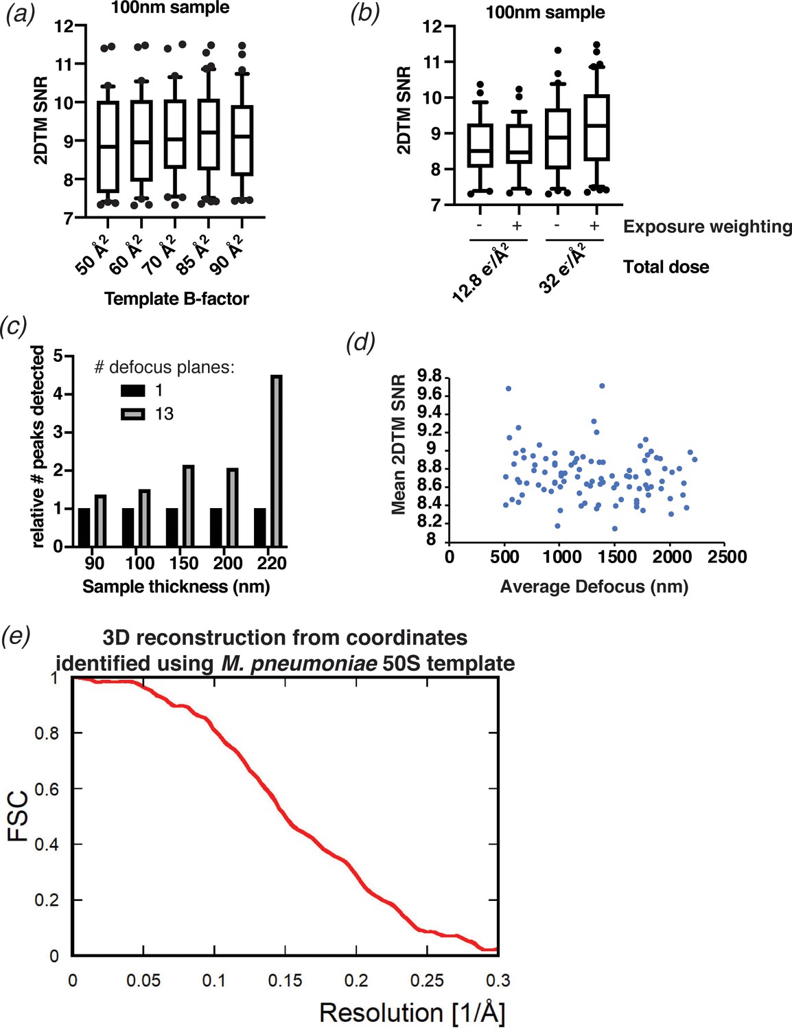
2DTM results obtained using different settings.
(a) Boxplot showing the distribution of 2DTM SNR values in a representative image using an M. pneumoniae 50S template with the indicated B-factor applied. The boxes indicate the interquartile range, the middle line indicates the median, the whiskers indicate the 10-90th percentiles and the dots indicate 50S peaks with SNRs outside this range. (b) As in (a), showing the distribution of 2DTM SNRs in images whereby 8 (12.8 e/Å2) or 20 (32 e/Å2) frames with or without exposure weighting were used to generate the final image as indicated. (c) Bar chart showing the number of detected 50S when 13 defocus planes are searched, relative to the number when a single defocus plane is searched. Individual images of indicated thickness are shown separately. (d) Scatterplot showing the mean 2DTM SNR of 50S identified in images with >10 peaks relative to the mean defocus of the image calculated using CTFFIND4. (e) FSC obtained for the 3D reconstruction (shown in Figure 3b) calculated from the targets found by 2DTM.
Figure 4 with 1 supplement

2DTM using a B. subtilis 50S template reveals species-specific structures.
(a) Molecular models of B. subtilis (red) and M. pneumoniae (blue) 50S ribosomal subunits aligned using UCSF Chimera (Pettersen et al., 2004). (b) Venn diagram showing the number of 50S subunits detected in the same dataset of 220 images of M. pneumoniae cells using the indicated template. (c) Boxplot showing the distribution of 2DTM SNR values of the locations quantified in the diagram in (b). The width of the box indicates the interquartile range, the middle line indicates the median and the whiskers indicate the range. The dashed vertical line indicates the 2DTM SNR threshold used. (d) 20 Å filtered 3D reconstruction generated using the locations and orientations of 1172 50S subunits detected in 220 images using 2DTM with a B. subtilis 50S template, showing clear density for the 30S ribosomal subunit and L7/L12 (not included in the template). The threshold was selected to reflect the threshold used in Figure 3b and c. (e) Difference map showing the regions of the 3D reconstructions that differ from the 50S 2DTM search template. Arrows indicate additional density consistent with 70S ribosome structures. (f) Difference map as described in (e) (gray mesh), aligned to the B. subtilis 50S template (red) and both M. pneumoniae (M.p., blue) and B. subtilis (red, not visible) molecular models. The difference map is shown at the same threshold as in (d). (g) 3D reconstruction as described in (d) (transparent gray), aligned to M. pneumoniae (M.p., blue) and B. subtilis (B.s., red) molecular models.
Figure 4—figure supplement 1
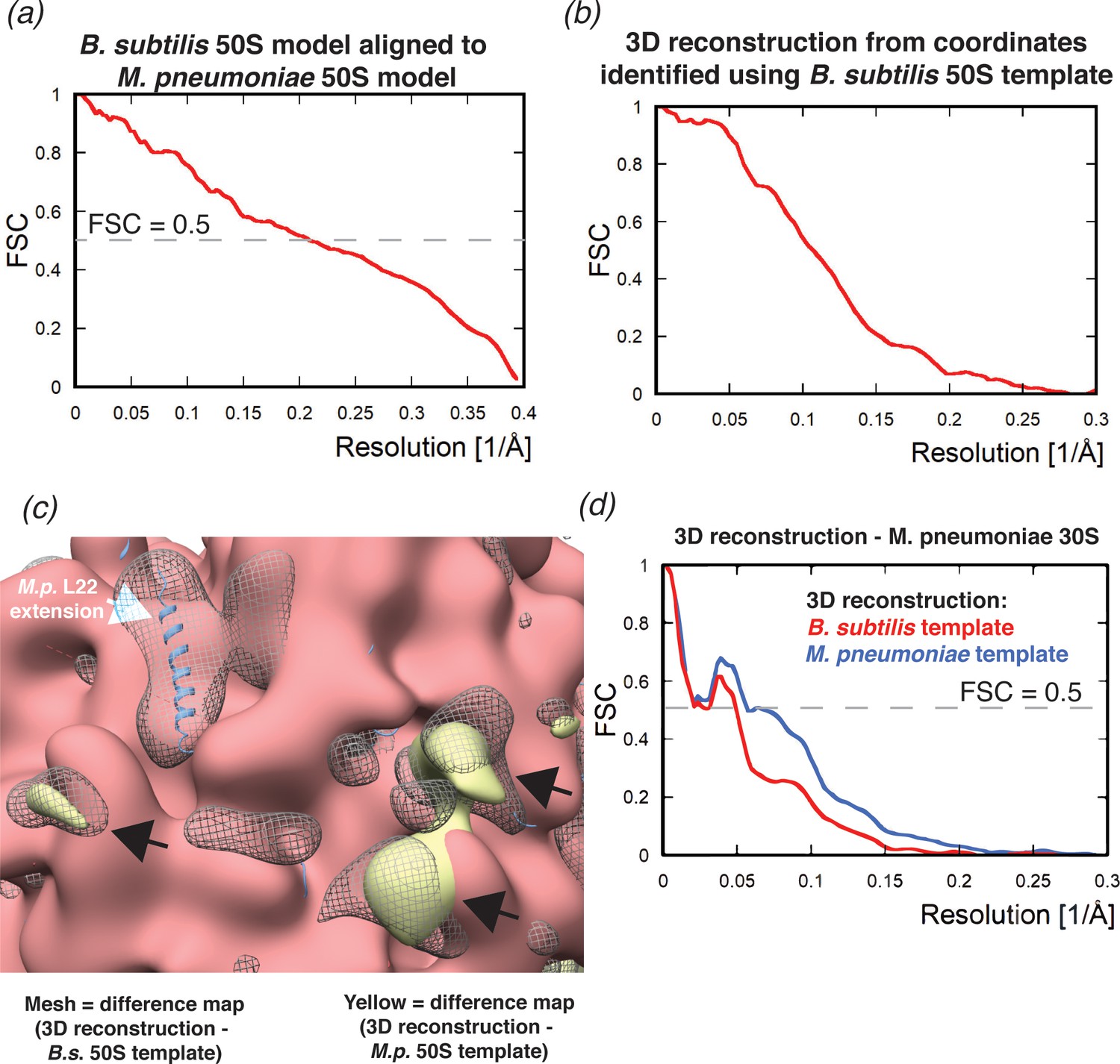
Comparison of 2DTM results using different 50S templates.
(a) FSC curve showing the correlation between the M.pneumoniae and B. subtilis templates. (b) FSC obtained for the 3D reconstruction calculated from the targets found by 2DTM (shown in Figure 4d). (c) Image showing the B. subtilis 50S template (red) aligned with the M. pneumoniae 50S model (blue), B. subtilis 50S model (not visible), the difference map from Figure 4e (gray mesh) and the difference map from Figure 3c. White arrow indicates the M. pneumoniae-specific C-terminal extension of L22, the black arrows indicate unattributed density that is common to both difference maps. (d) FSC curves showing the correlation between the 3D reconstructions generated from the targets identified with the indicated 50S templates and masked in the area of the 30S subunit, and the M. pneumoniae 30S structure. The 0.5 threshold indicates the resolution limit in each case.
Figure 5 with 2 supplements

Comparison of ribosome detection by 2DTM and 3DTM.
(a) Images of untilted cryo-EM grids of M. pneumoniae were collected with a total exposure of 32 e-/Å2, followed by a tilt series of an overlapping region with a total exposure of 129 e-/Å2 to reconstruct a tomogram. (b) 50S ribosomal subunits were identified in the 2D images by 2DTM with the M. pneumoniae 50S (left) and in the 3D tomogram by 3DTM using the 50S subunit as a template (right). The 2DTM and 3DTM templates were aligned to ensure that the respective coordinate systems were aligned, and that the x,y coordinates of the detected 50S subunits in each search could be aligned. (c) The proportion of 2DTM and 3DTM coordinates within 100 Å and 20° in each of the three Euler angles in 19 images was calculated using an SNR threshold that allowed either one false positive per image (upper), or detection of ~2 times more potential 50S targets (lower). (d) Plot showing the proportion of 2DTM targets that were also detected by 3DTM as a function of sample thickness. (e) Plot showing the proportion of 3DTM targets that were also detected by 2DTM as a function of sample thickness. (f) Plot showing the proportion of 2DTM 50S targets with a positional and rotational 3DTM match at the indicated 2DTM SNR threshold (dashed line). (g) Plot showing the number of expected false positives in the 2DTM search assuming a Gaussian noise model (black) and the observed number of 2DTM targets without a matching 3DTM target (blue) at the indicated 2DTM SNR.
Figure 5—figure supplement 1
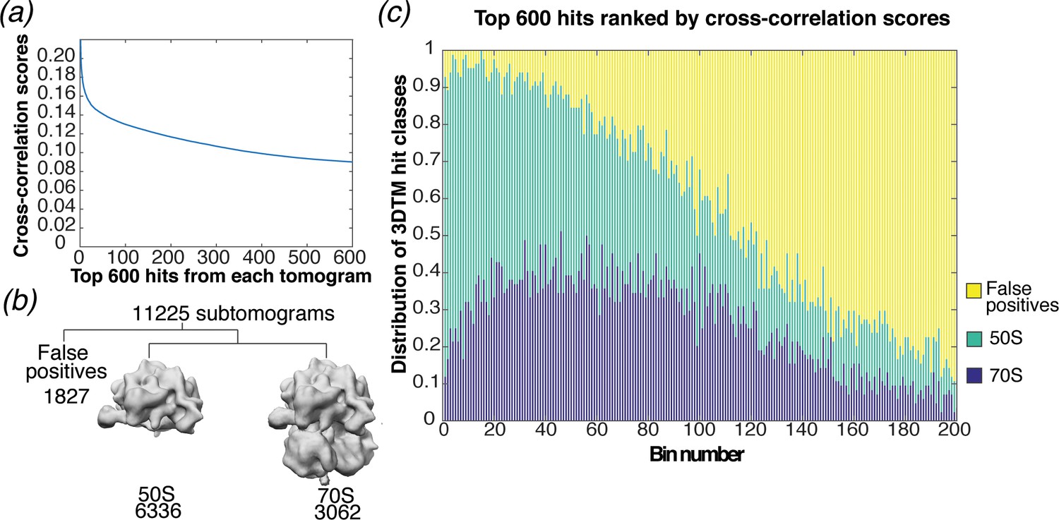
Analysis of targets detected by 3DTM.
(a) Cross-correlation scores for the top 600 hits detected in 3DTM using a 50S template. (b) Classification of the subtomograms in RELION. (c) Bar chart showing the proportion of ranked 3DTM hits classified as false positives (yellow), 50S (green; used as a template) or 70S (purple) by classification in RELION. The ranked hits are binned in sets of 3.
Figure 5—figure supplement 2
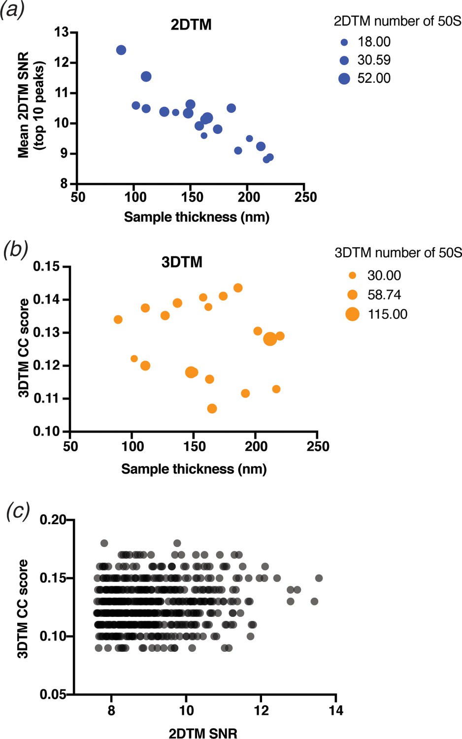
Comparison of 2DTM and 3DTM results.
(a) Scatterplot showing the mean 2DTM SNR of the 19 images searched in Figure 5 relative to the sample thickness calculated from a tomogram. The size of each point is proportional to the total number of 50S detected with 2DTM as shown in the legend (right). (b) As in (a), showing the number of 50S detected with 3DTM in the area of the tomogram overlapping the 2D image. (c) Scatterplot showing the 2DTM SNR relative to the 3DTM cross-correlation (CC) score of all 576 targets identified in Figure 5.
Figure 6 with 1 supplement
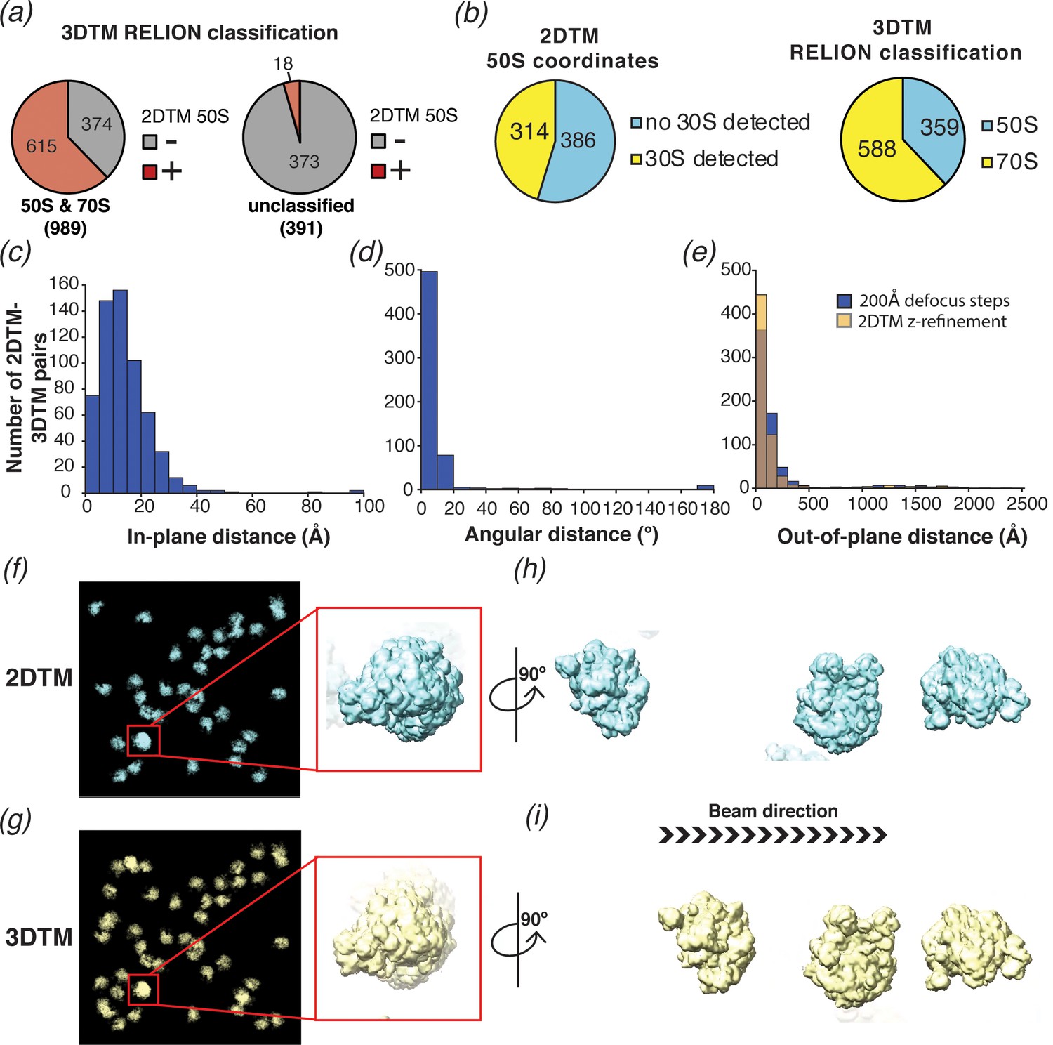
2DTM is precise, excludes non-ribosome particles and permits detection of ribosomes overlapping along the projection direction.
(a) Pie chart showing the results of a comparison of a set of 1380 3DTM coordinates initially identified by PyTom followed by 3D classification in RELION that identified 989 targets as 50S or 70S (left) and 391 targets as non-ribosomal particles (right), with a list of 652 50S 2DTM targets. Red indicates the proportion aligning with 50S coordinates identified by 2DTM; gray indicates non-matching 3DTM coordinates. (b) Pie charts showing the proportion of 50S detected by 2DTM with the M. pneumoniae template with a bound 30S target as determined by performing a local search with refine_template (see Materials and methods) (left), and the ratio of 3DTM 50S targets classified as 70S or 50S by RELION (right). (c) Histogram showing the distribution of the in-plane distance between matched 3DTM and 2DTM after 3DTM refinement of the subtomograms with RELION. (d) As in (c), showing the angular distance. (e) As in (c), showing the out-of-plane difference (z coordinate) before (blue) or after (yellow) 2DTM refinement of z coordinates. (f) Plotted result from a 2DTM search showing template projections at the locations and Euler angles of detected 50S subunits (left), inset showing two overlapping 50S subunits when viewed parallel to the image plane. (g) As in (f), showing the plotted result from 3DTM of the same area aligned to show the same perspective. (h) The template projections in (f) rotated 90° to show the overlapping 50S subunits perpendicular to the image plane. (i) As in (h), showing the result from 3DTM in the same area.
Figure 6—figure supplement 1
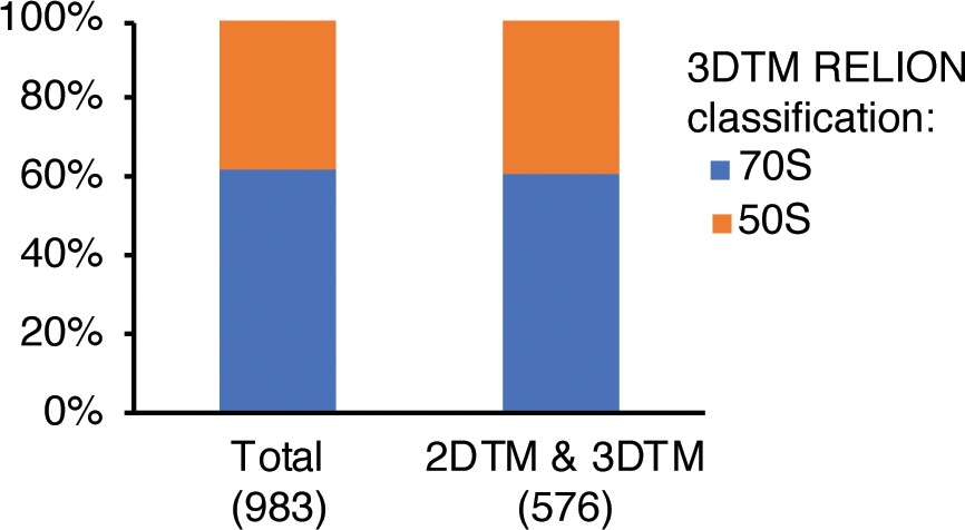
Proportional bar chart showing the percentage of all 983.
3DTM targets in the area of the tomogram overlapping with the 2D image, and the 576 3DTM targets that were also detected by 2DTM, indicating 50S (orange) or 70S (blue) in each case as classified by RELION.
Tables
Key resources table
| Reagent type (species) or resource | Designation | Source or reference | Identifiers | Additional information |
|---|---|---|---|---|
| Cell line (Mycoplasma pneumonia) | M129 | O'Reilly et al., 2020 | ATCC 29342 | |
| Software, algorithm | cisTEM | This paper and Grant Grant et al., 2018. | doi:10.5281/zenodo.4603401 | https://cistem.org/ |
Additional files
Download links
A two-part list of links to download the article, or parts of the article, in various formats.
Downloads (link to download the article as PDF)
Open citations (links to open the citations from this article in various online reference manager services)
Cite this article (links to download the citations from this article in formats compatible with various reference manager tools)
Locating macromolecular assemblies in cells by 2D template matching with cisTEM
eLife 10:e68946.
https://doi.org/10.7554/eLife.68946


