An automated feeding system for the African killifish reveals the impact of diet on lifespan and allows scalable assessment of associative learning
- Department of Genetics, Stanford University, United States
- Biology Graduate Program, Stanford University, United States
- Department of Neurology and Neurological Sciences, Stanford University, United States
- Neurosciences Interdepartmental Program, Stanford University School of Medicine, United States
- Department of Bioengineering, Stanford University, United States
- Thielvoldt Engineering, United States
- Glenn Laboratories for the Biology of Aging, Stanford University, United States
- Wu Tsai Neurosciences Institute, Stanford University, United States
Figures
Figure 1 with 2 supplements
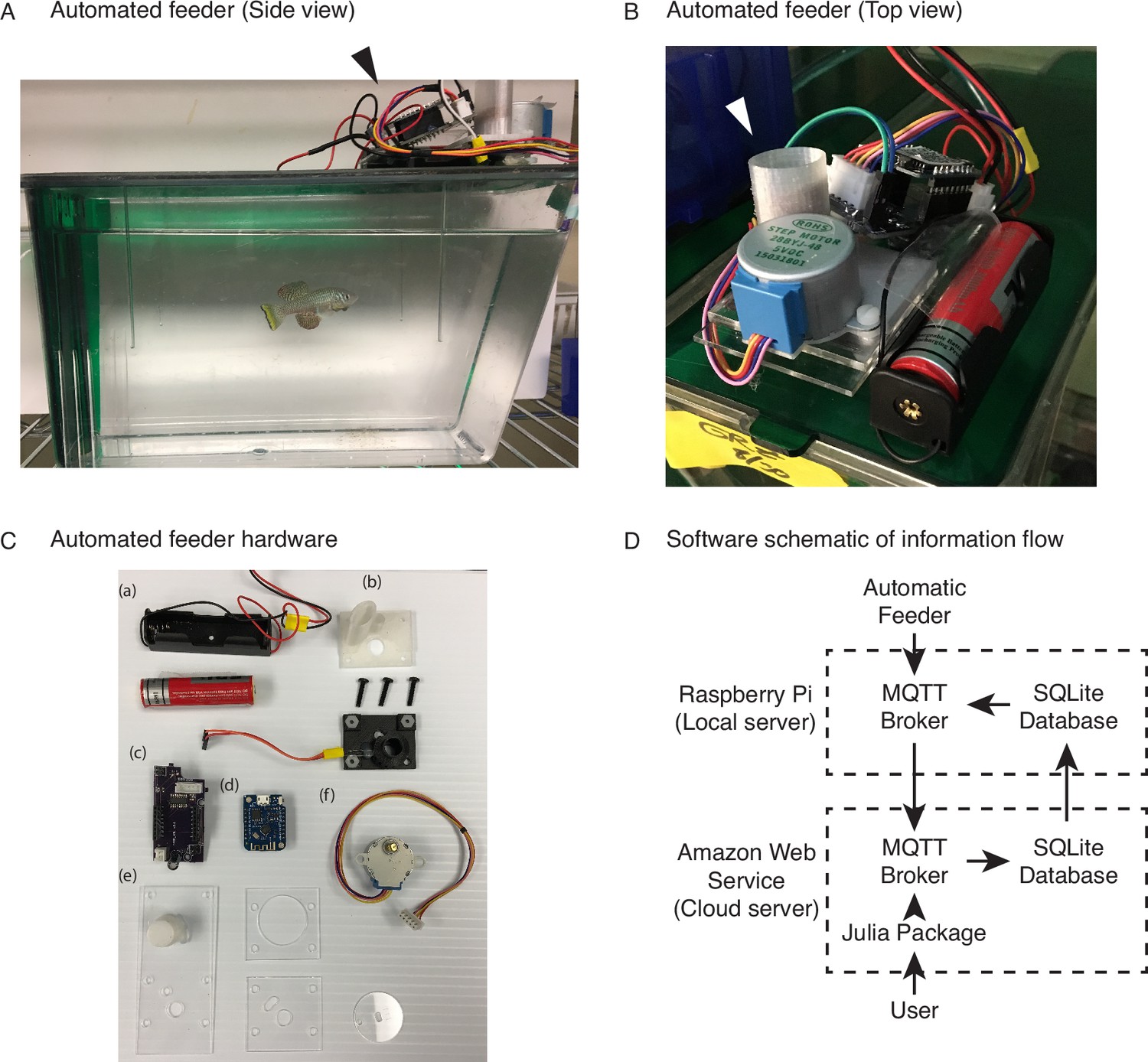
An automated 3D-printed feeding system for the African turquoise killifish.
(A) Side view of an individual automated feeding unit placed on the top front of a 2.8 L fish tank supplied by Aquaneering. At the midpoint of the tank height, a 2.8 L tank is approximately 23 cm long from front to back. Dark arrowhead: feeding unit on the lid of a tank. (B) Top view of an individual automated feeding unit. This is a compact, self-contained unit with individual power supply, food hopper, stepper motor for food delivery, and microcontroller for control and communication. White arrowhead: hopper where the dry food is placed. (C) Components of an individual automated feeder. Each feeder is composed of a lithium ion battery and holder (a), 3D-printed parts (b) coupled with a custom-printed circuit board (c), a Wemos D1 mini ESP8266-based microcontroller board (d), laser-cut acrylic parts (e), and stepper motor (f). (D) Users control the automated feeding system by interacting with a cloud-based server. This server communicates with small local servers on the premise, which then communicate with the individual automated feeders. Changes to feeding schedules are provided by users and filter down to the appropriate feeders, while status updates, such as feeding confirmations, make the return trip back to the users.
-
Figure 1—source data 1
Automatic feeder parts list.
- https://cdn.elifesciences.org/articles/69008/elife-69008-fig1-data1-v2.xlsx
Figure 1—figure supplement 1
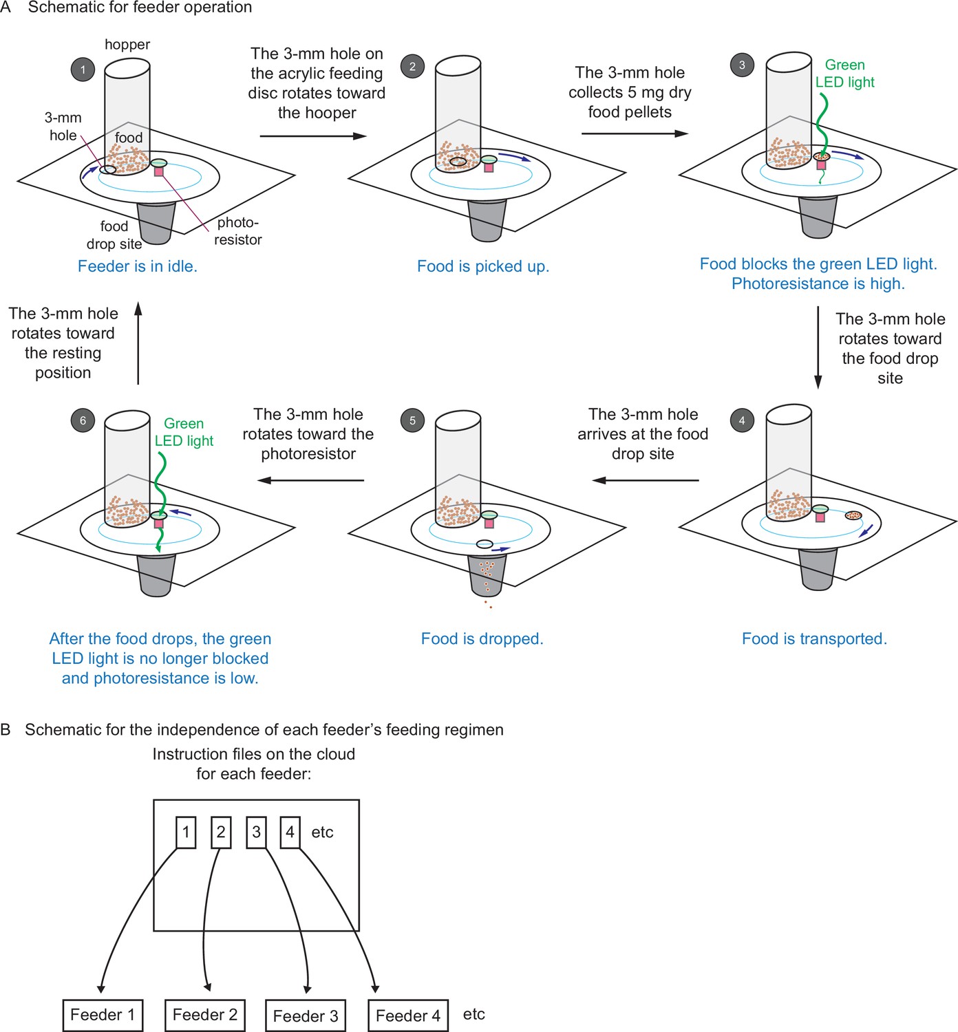
Automated feeders are designed to confirm each feeding and can be programmed to perform independent feeding regimens.
(A) Schematic showing how the automated feeder operates. Step 1, at the programmed feeding time, the feeder wakes up from idle and receives the operation instruction from the network. The 3-mm hole turns toward the hopper. Step 2, the 3-mm hole collects 5 mg of dry food from the hopper. Step 3, the 3-mm hole sits on top of the photoresistor. Because the food blocks the green light-emitting diode (LED) light from reaching the photoresistor, a high value of photoresistance is recorded on the network. Step 4, the 3-mm hole carries the food toward the food drop site. Step 5, the 3-mm hole arrives at the food drop site and drops food. Then it returns to the photoresistor. Step 6, after food drops, the green LED light is no longer blocked, and a low value of photoresistance is recorded on the network. Then the 3-mm hole moves back to the resting position until next feeding. The change in photoresistance between steps 3 and 6 indicates that the food has been dropped. (B) Schematic showing that each feeder can be programmed with separate and independent feeding regimens. Each feeder has a unique ID (associated with each Wemos D1 mini ESP8266-based development board), along with an individual set of instructions stored on the server that can be updated independently of every other feeder. This setup allows different feeding regimens to be implemented simultaneously for different tanks.
Figure 1—video 1
Example of automatic feeder function.
Figure 2 with 1 supplement

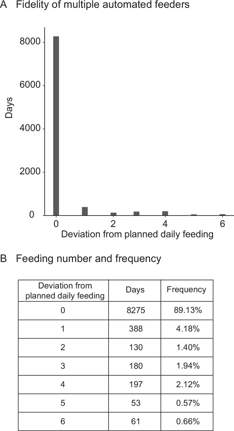
Fidelity and precision of the automated feeding system.
(A) Logged feedings per day from a representative feeder over a 30-day period, with seven feedings of 5 mg programmed for each day. Note that a recording of six feedings instead of seven does not necessarily mean that the feeding was missed but could be due to an unlogged feeding due to inability to connect to main server. Source data: Figure 2—source data 1. (B, C) Histogram (B) of deviations from scheduled feedings for 2279 days of feedings over 41 feeders with a given number of deviations tabulated in (C). The vast majority (>98%) of feedings have zero or one missed feeding. Source data: Figure 2—source data 2. (D) Automated feeding provides higher feeding precision than manual feeding as seen from the dispersion of feeding volumes as a percentage of the mean. When compared to manual feeding by multiple individual users or a single individual, automated feeders are more precise in the amount of food delivered. Precision is defined as the reciprocal of the estimated variance given either six individuals (n = 54, precision = 0.016), one individual (n = 9, precision = 0.082), four feeders (n = 19, precision = 0.512), or one single feeder (n = 10, precision = 0.559). Precision derived from bootstrapped estimates of the standard deviation for each group. Source data: Figure 2—source data 3.
-
Figure 2—source data 1
Feeding logs from a representative feeder over a 30-day period.
- https://cdn.elifesciences.org/articles/69008/elife-69008-fig2-data1-v2.csv
-
Figure 2—source data 2
Missed feedings for 41 feeders over 2279 days of feeding.
- https://cdn.elifesciences.org/articles/69008/elife-69008-fig2-data2-v2.csv
-
Figure 2—source data 3
Feeding data for automatic and manual feedings.
- https://cdn.elifesciences.org/articles/69008/elife-69008-fig2-data3-v2.csv
-
Figure 2—source data 4
Missed feedings for 90 feeders over 9284 days of feeding.
- https://cdn.elifesciences.org/articles/69008/elife-69008-fig2-data4-v2.csv
Figure 2—figure supplement 1
Fidelity and precision of the automated feeding system validated by independent researcher.
(A) Histogram of deviations from scheduled feedings for 9284 days of feedings over 90 feeders. The vast majority (>94%) of feedings have zero or one missed feeding. Source data: Figure 2—source data 4. (B) Deviations from scheduled feedings for 9284 days of feedings over 90 feeders with a given number of deviations tabulated. Source data: Figure 2—source data 4.
Figure 3 with 1 supplement
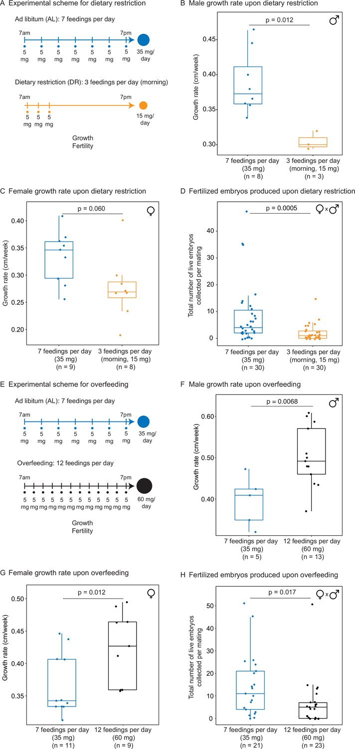
Automated feeding enables the definition of different diets for the African killifish.
(A) Experimental scheme to compare two automated feeding schedules for killifish: feeding seven times a day evenly over 12 hr (5 mg Otohime fish diet per feeding, 35 mg total per day) and feeding three times a day within a 2 hr period in the morning (5 mg Otohime fish diet per feeding, 15 mg total per day). These regimens were applied from 1 month of age to death (for growth measurements) and from 1 month of age until death of one individual in the pair (for fertility measurements). For fertility measurements, each individual in the pair was fed individually while single-housed and then crossed for 24 hr once per week to assess fertility. (B) The average growth rate (cm/week) of male killifish from 1 month of age to death fed either seven times a day (blue, median = 0.3726 cm/week, n = 8) is significantly greater than those fed three times a day in the morning (orange, median = 0.3 cm/week, n = 3). Each dot represents a single animal’s growth averaged over its lifespan. Animals that lived longer than 4 months were not considered due to concerns with nonlinear growth rate. Significance determined by Wilcoxon rank-sum test (p=0.012). Animals were from the same cohort as Figure 4—figure supplement 1 (cohort 1). Source data: Figure 3—source data 1. (C) The average growth rate (cm/week) of female killifish from 1 month of age to death fed seven times a day (blue, median = 0.3461 cm/week, n = 9) is greater than those fed three times a day in the morning (orange, median = 0.2690 cm/week, n = 8). Each dot represents a single animal’s growth averaged over their lifespan. Animals that lived longer than 4 months were not considered due to concerns with nonlinear growth rate. Significance determined by Wilcoxon rank-sum test (p=0.060). Animals were from the same cohort as Figure 4—figure supplement 1 (cohort 1). Source data: Figure 3—source data 1. (D) Killifish mating pairs (one male and one female) fed three times a day are significantly less fertile (median = 1 fertilized embryo per mating, n = 30 matings across five pairs) than mating pairs fed seven times a day (median = 4 fertilized embryos per mating, n = 30 matings across five pairs). Each dot represents the fertilized embryos collected from one pair crossing overnight, and pairs were mated from 8 weeks of age until one individual in the pair died. Significance determined by Wilcoxon rank-sum test (p=0.0005). Source data: Figure 3—source data 2 and Figure 3—source data 3. (E) Experimental scheme to compare two automated feeding schedules for killifish: feeding twelve times a day (5 mg Otohime fish diet per feeding, 60 mg total per day) compared to feeding seven times a day (5 mg Otohime fish diet per feeding, 35 mg total per day). These regimens were applied from 1 month of age to death (for growth measurements) and from 2 months of age until death of one individual in the pair (for fertility measurements). For fertility measurements, each individual in the pair was fed individually while single-housed and then crossed for 24 hr once per week to assess fertility. (F) The average growth rate (cm/week) of male killifish from 1 month of age to death is significantly higher for animals fed twelve times a day (black, median = 0.4917 cm/week, n = 13 males) than for animals fed seven times a day (blue, median = 0.4092 cm/week, n = 5 males). Each dot represents a single animal’s growth averaged over its lifespan. Animals that lived longer than 4 months were not considered due to concerns with nonlinear growth rate. Significance determined by Wilcoxon rank-sum test (p=0.0068). Source data: Figure 3—source data 4. (G) The average growth rate (cm/week) of female killifish from 1 month of age to death is significantly higher for animals fed twelve times a day (black, median = 0.4268 cm/week, n = 9 females) than for animals fed seven times a day (blue, median = 0.3425 cm/week, n = 11 females). Each dot represents a single animal’s growth averaged over its lifespan. Animals that lived longer than 4 months were not considered due to concerns with nonlinear growth rate. Significance determined by Wilcoxon rank-sum test (p=0.012). Source data: Figure 3—source data 4. (H) Killifish mating pair fertility is significantly lower for animals fed twelve times a day (black feeding schedule, median = 5 fertilized embryos per mating, n = 23 matings) than for animals fed seven times a day (blue feeding schedule, median = 11 fertilized embryos per mating, n = 21 matings). Each dot represents fertilized embryos collected from one pair upon crossing for 24 hr and pairs were mated from 2 months of age until one individual in the pair died. Significance determined by Wilcoxon rank-sum test (p=0.017). Source data: Figure 3—source data 5 and Figure 3—source data 6.
-
Figure 3—source data 1
Metadata table for growth rate comparisons for males and female killifish on dietary restriction (DR) diet regimens.
- https://cdn.elifesciences.org/articles/69008/elife-69008-fig3-data1-v2.csv
-
Figure 3—source data 2
Embryo viability data for mate pairs on dietary restriction (DR) or ad libitum (AL) diet regimens.
- https://cdn.elifesciences.org/articles/69008/elife-69008-fig3-data2-v2.csv
-
Figure 3—source data 3
Metadata table for mate pairs used in embryo viability experiments in Figure 3—source data 2.
- https://cdn.elifesciences.org/articles/69008/elife-69008-fig3-data3-v2.csv
-
Figure 3—source data 4
Metadata table for growth rate comparisons for males and female killifish on OE diet regimens.
- https://cdn.elifesciences.org/articles/69008/elife-69008-fig3-data4-v2.csv
-
Figure 3—source data 5
Embryo viability data for mate pairs on overfeeding or ad libitum (AL) diet regimens.
- https://cdn.elifesciences.org/articles/69008/elife-69008-fig3-data5-v2.csv
-
Figure 3—source data 6
Metadata table for mate pairs used in embryo viability experiments in Figure 3—source data 5.
- https://cdn.elifesciences.org/articles/69008/elife-69008-fig3-data6-v2.csv
Figure 3—figure supplement 1
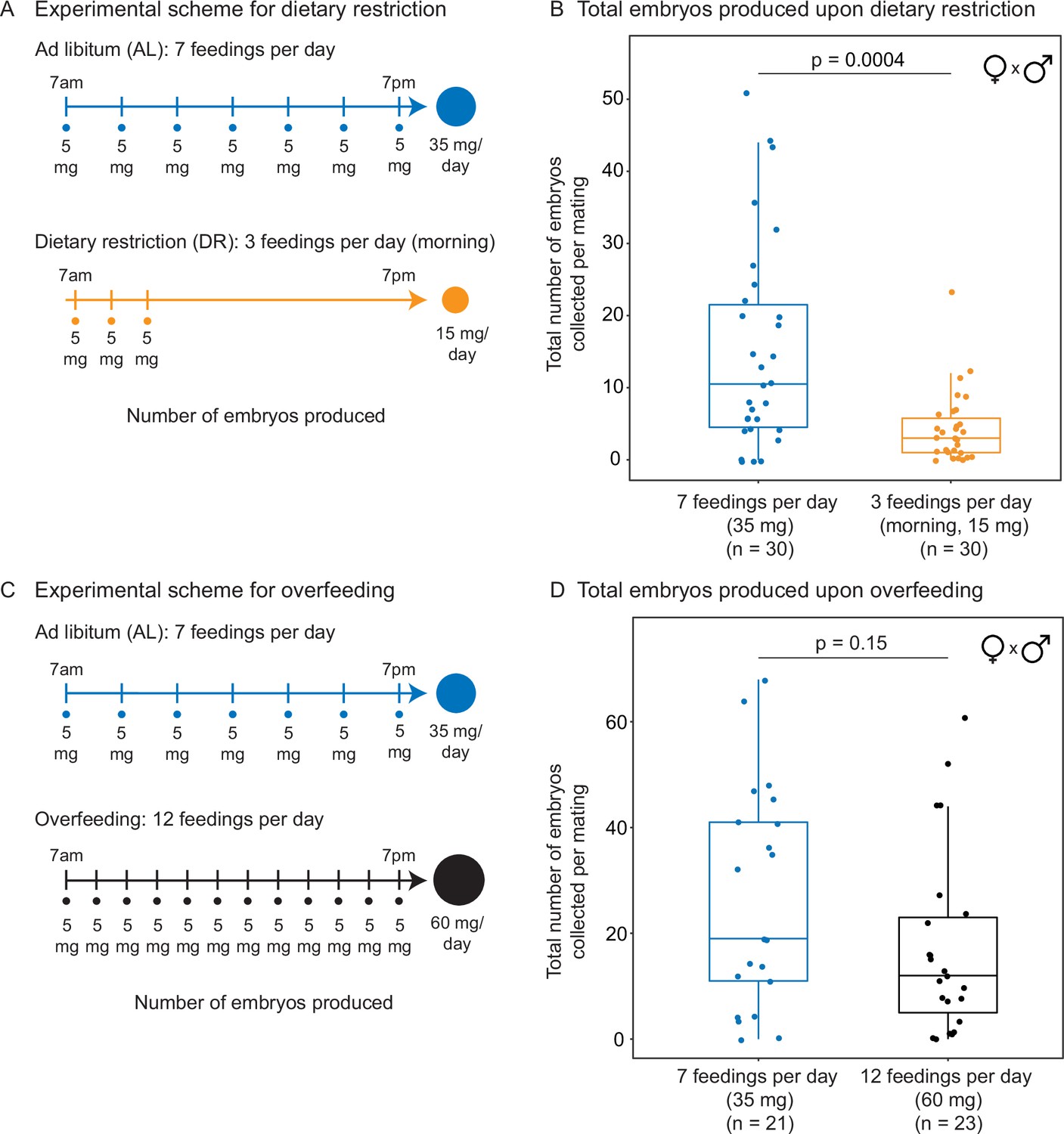
Total number of embryos produced in response to different diets.
(A) Experimental scheme to compare two automated feeding schedules for killifish: feeding seven times a day evenly over 12 hr (5 mg Otohime fish diet per feeding, 35 mg total per day) and feeding three times a day within a 2 hr period in the morning (5 mg Otohime fish diet per feeding, 15 mg total per day). These regimens were applied from 1 month of age until death of one individual in the pair. Each individual in the pair was fed individually while single-housed and then crossed for 24 hr once per week to assess number of embryos produced. (B) Killifish mating pairs fed three times a day produce significantly fewer total embryos (median = 3 total embryos per mating, n = 30 matings across five pairs) than mating pairs fed seven times a day (median = 10.5 total embryos per mating, n = 30 matings across five pairs). Each dot represents the total embryos collected from one pair crossing overnight. Significance determined by Wilcoxon rank-sum test (p=0.0004). Source data: Figure 3—source data 2 and Figure 3—source data 3. (C) Experimental scheme to compare two automated feeding schedules for killifish: feeding twelve times a day (5 mg Otohime fish diet per feeding, 60 mg total per day) compared to feeding seven times a day (5 mg Otohime fish diet per feeding, 35 mg total per day). These regimens were applied from 2 months of age until death of one individual in the pair. Each individual in the pair was fed individually while single-housed and then crossed for 24 hr once per week to assess the number of embryos produced. (D) Killifish mating pairs fed twelve times a day do not produce significantly fewer total embryos (black feeding schedule, median = 12 total embryos per mating, n = 23 matings, across three pairs) than for those fed seven times a day (blue feeding schedule, median = 19 total embryos per mating, n = 21 matings across three pairs). Each dot represents the total embryos collected from one pair crossing overnight. Significance determined by Wilcoxon rank-sum test (p=0.15). Source data: Figure 3—source data 5, Figure 3—source data 6.
Figure 4 with 1 supplement
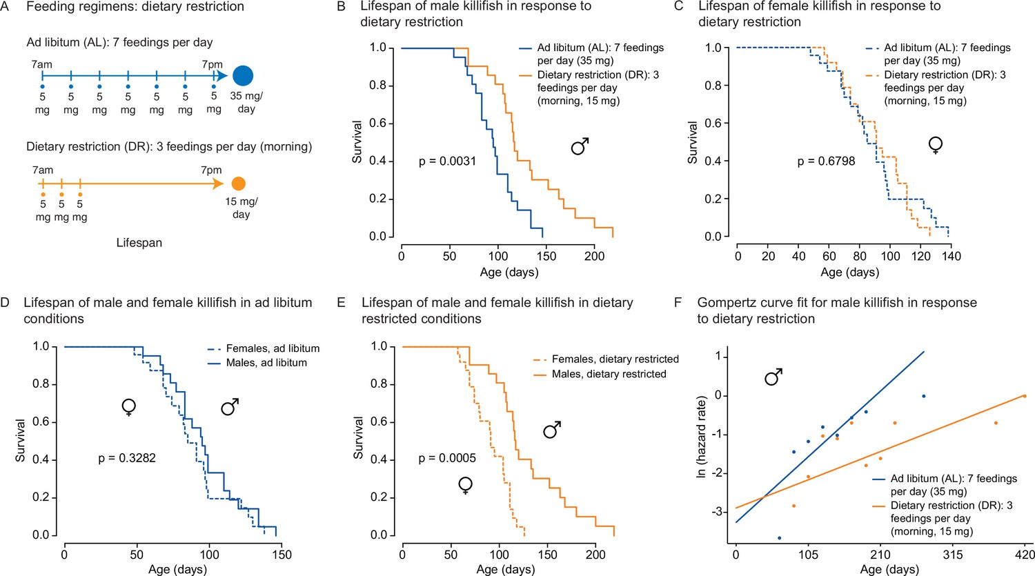
An amount- and time-restricted dietary regimen robustly extends lifespan in male, but not female African turquoise killifish.
(A) Experimental scheme comparing two automated feeding schedules for killifish: an ad libitum (AL) regimen (seven times a day, 35 mg Otohime fish diet per day, blue) or a dietary restricted (DR) regimen (three times in the morning, 15 mg Otohime fish diet per day, orange). Automated feeding regimens were started after sexual maturity, at 1 month of age. (B) Male killifish fed a DR regimen (solid orange, median lifespan = 116 days, n = 21) lived significantly longer than male killifish fed an AL regimen (solid blue, median lifespan = 95 days, n = 21) (p=0.0031, log-rank test). Source data: Figure 4—source data 1. (C) Female killifish fed a DR regimen (dashed orange, median lifespan = 90 days, n = 25) did not live significantly longer than female killifish fed an AL regimen (dashed blue, median lifespan = 82.5 days, n = 24) (p=0.6798, log-rank test). Source data: Figure 4—source data 1. (D) In AL conditions, male killifish (solid blue, median lifespan = 95 days, n = 21) did not exhibit lifespan difference from female killifish (dashed blue, median lifespan = 82.5 days, n = 24) (p=0.3282, log-rank test). Source data: Figure 4—source data 1. (E) In DR conditions, male killifish (solid orange, median lifespan = 116 days, n = 21) lived significantly longer than female killifish (dashed orange, median lifespan = 90 days, n = 25) (p=0.0005, log-rank test). Source data: Figure 4—source data 1. (F) Fitted curve of the binned 27-day hazard rate of male killifish from both cohorts to a Gompertz distribution and then transformed into the natural log of the hazard rate. The estimated ‘rate of aging’ (slope) of killifish on the AL feeding regimen is 0.3388 (95% confidence interval = 0.2437–0.434) and is significantly different from the rate of aging for DR, which is 0.1457 (95% confidence interval = 0.0846–0.2069). The estimated ‘frailty’ (intercept) for killifish on the AL feeding regimen is 0.0385 (95% confidence interval = 0.0203–0.073) compared to 0.0557 (95% confidence interval = 0.0315–0.0986) for killifish on DR (overlapping confidence intervals for intercept parameter indicate that these parameters are not significant). Source data: Figure 4—source data 1 and Figure 4—source data 2.
-
Figure 4—source data 1
Lifespan data for male and female killifish on ad libitum (AL) and dietary restriction (DR) diet regimens (cohort 2).
- https://cdn.elifesciences.org/articles/69008/elife-69008-fig4-data1-v2.csv
-
Figure 4—source data 2
Lifespan data for male and female killifish on ad libitum (AL) and dietary restriction (DR) diet regimens from independent cohort (cohort 1).
- https://cdn.elifesciences.org/articles/69008/elife-69008-fig4-data2-v2.csv
-
Figure 4—source data 3
Result from proportional hazards model that shows dietary restriction (DR) independently and significantly reduces the hazard rate.
- https://cdn.elifesciences.org/articles/69008/elife-69008-fig4-data3-v2.xlsx
Figure 4—figure supplement 1
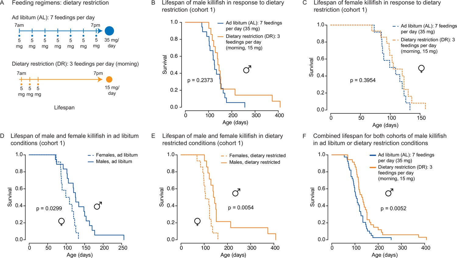
An independent cohort of African turquoise killifish undergoing the amount- and time-restricted dietary regimen also exhibits lifespan extension in males.
(A) Experimental scheme comparing two automated feeding schedules for killifish: an ad libitum (AL) regimen (seven times a day, 35 mg Otohime fish diet per day, blue) or a dietary restricted (DR) regimen (three times in the morning, 15 mg Otohime fish diet per day, orange). Feeding was started after sexual maturity, at 1 month of age. (B) In an independent cohort (cohort 1), male killifish fed a DR regimen (solid orange, median lifespan = 142.5 days, n = 15) did not live significantly longer than male killifish fed an AL regimen (solid blue, median lifespan = 125.5 days, n = 21) (p=0.2373, log-rank test). Source data: Figure 4—source data 2. (C) In an independent cohort (cohort 1), female killifish fed an amount- and time-restricted dietary regimen (dashed orange, median lifespan = 104 days, n = 18) did not live significantly longer than female killifish fed an AL regimen (dashed blue, median lifespan = 104 days, n = 14) (p=0.3954, log-rank test). Source data: Figure 4—source data 2. (D) In an independent cohort (cohort 1) with AL conditions, male killifish (solid blue, median lifespan = 125.5 days, n = 21) did exhibit a lifespan difference from female killifish (dashed blue, median lifespan = 104 days, n = 14) (p=0.0299, log-rank test). Source data: Figure 4—source data 2. (E) In an independent cohort (cohort 1) with DR conditions, male killifish (solid orange, median lifespan = 142.5 days, n = 15) lived significantly longer than female killifish (dashed orange, median lifespan = 104 days, n = 18) (p=0.0054, log-rank test). Source data: Figure 4—source data 2. (F) Combining the lifespans of the first and second cohorts of male killifish, we found the additional animals did not change the conclusion from the second cohort that male killifish on an AL diet (solid blue, median lifespan = 106 days, n = 42) live significantly shorter than DR animals (dashed orange, median lifespan = 129 days, n = 36) (p=0.0052, log-rank test). Source data: Figure 4—source data 1 and Figure 4—source data 2.
Figure 5 with 1 supplement
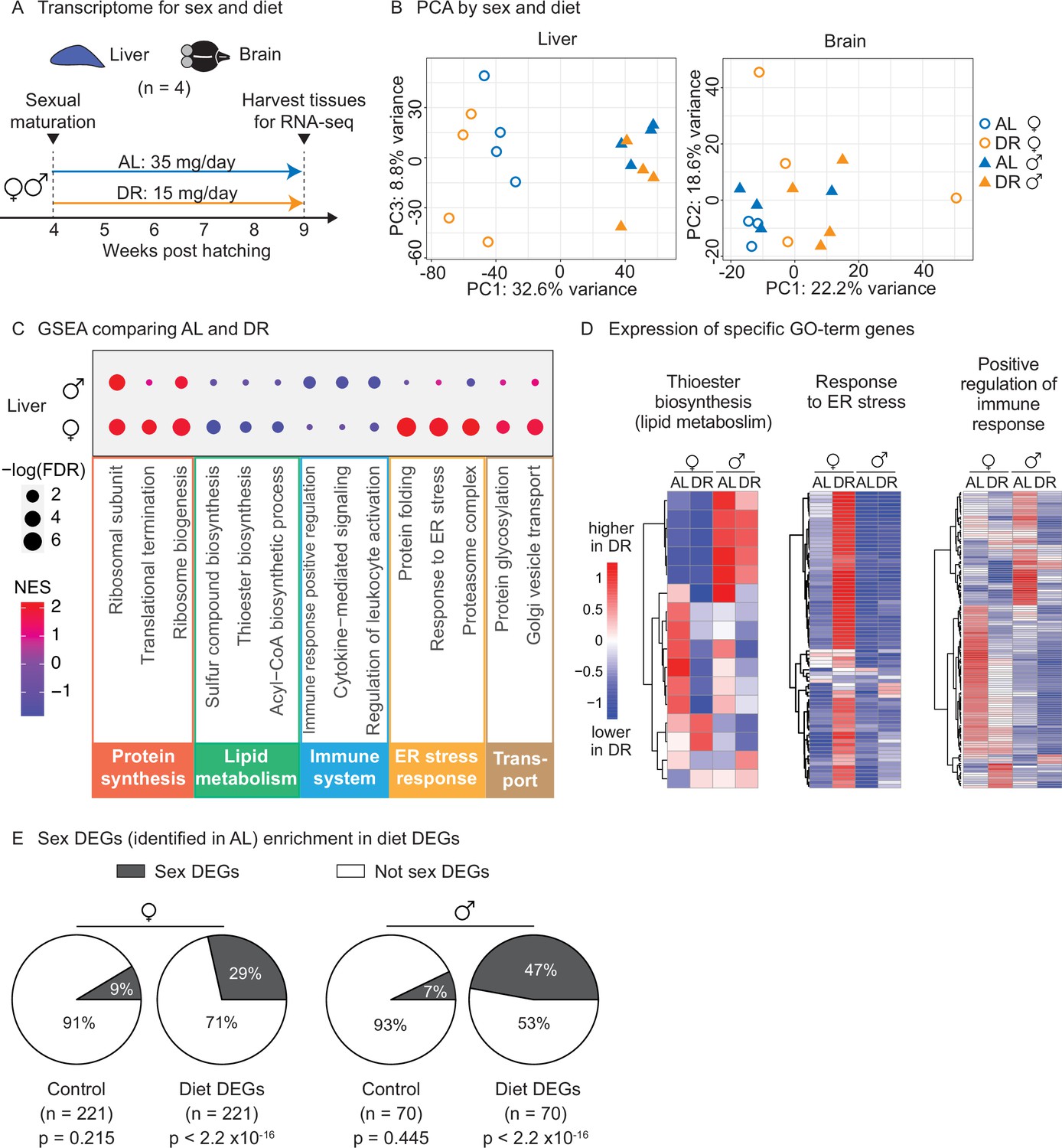
Transcriptomic analysis shows that an amount- and time-restricted dietary restriction (DR) induces sex-specific gene expression in the liver of the killifish.
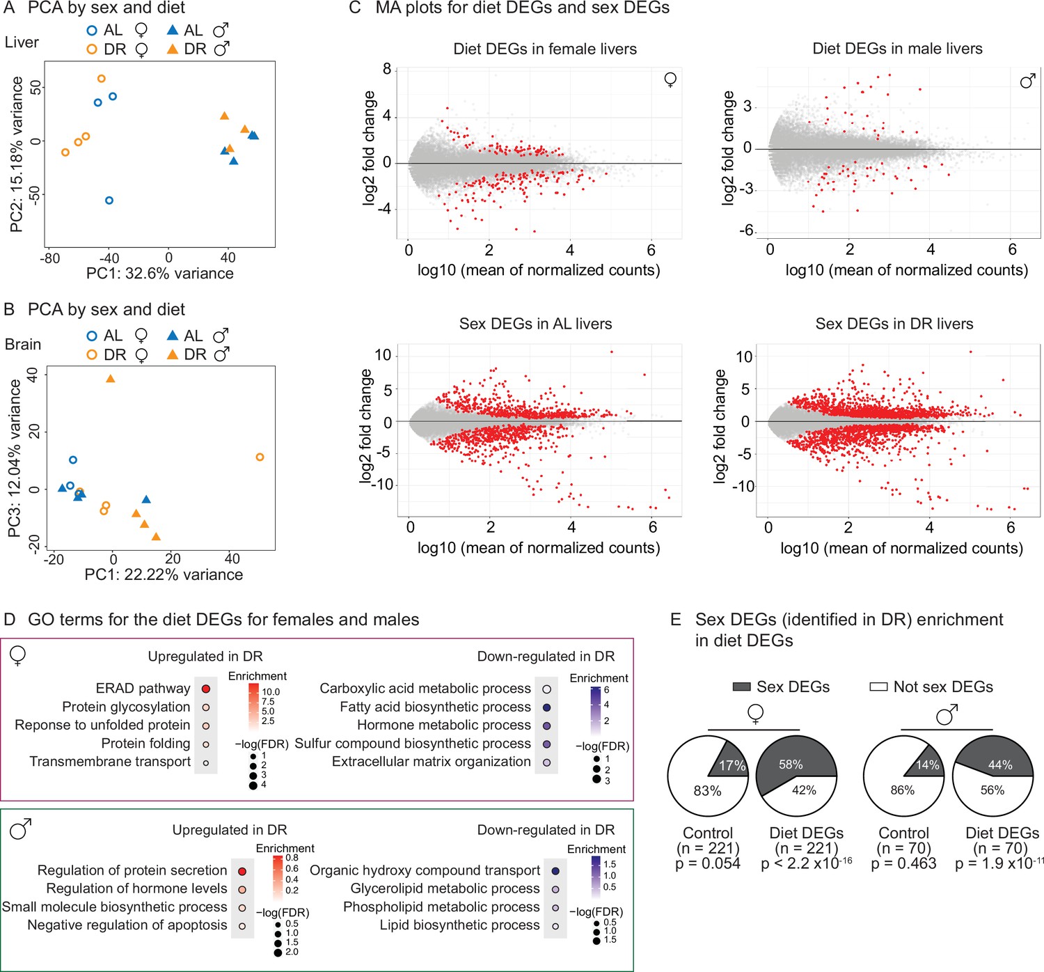
(A) Experimental scheme to compare the liver and brain transcriptomes in ad libitum (AL) or DR conditions for males and females. A 5-week amount- and time-restricted DR regimen was used (similar to Figure 4) and four animals per sex (n = 4) were used. (B) Principal component analysis (PCA) of the transcriptomes of all liver samples (PC1 and PC3), or brain samples (PC1 and PC2), with samples coded by sex and diet regimens. For other PCs, see Figure 5—figure supplement 1A and B. Variance stabilization transformation was applied to the raw counts, and the transformed count data were used as PCA input. Each symbol represents the full transcriptome of one individual fish. (C) Selected gene set enrichment analysis (GSEA) results, comparing the AL and DR liver transcriptomes for males and females. Dot color represents the normalized enrichment score of each GO term. Red, higher expression in DR; blue, lower expression in DR. Dot size represents the –log10 of the adjusted p-value (i.e., false discovery rate [FDR] after multiple hypotheses testing). (D) Average scaled expression of the genes underlying specific GO terms for the liver. The average scaled expression of the four replicates per condition (Female AL; Female DR, Male AL; Male DR) was plotted in the heatmaps (see ‘Materials and methods’). Red, higher expression in DR; blue, lower in DR. (E) Sex differentially expressed genes (DEGs) (identified in AL livers) were enriched in diet DEGs, for both males and females. The non-diet DEGs control gene set (‘control’) and the diet DEGs shared the same transcript expression distribution and gene group size (see ‘Materials and methods’). The percentage of genes being sex DEGs for each gene set (‘enrichment’) was plotted as pie charts. The number of genes in each gene set (n) is indicated in parentheses. Significance determined by a two-tailed Fisher’s exact test. For the control gene sets, the median p-value and enrichment in the bootstrapped results were reported.
-
Figure 5—source data 1
Experimental metadata for bulk RNA-sequencing experiments.
- https://cdn.elifesciences.org/articles/69008/elife-69008-fig5-data1-v2.xlsx
-
Figure 5—source data 2
Diet differentially expressed gene (DEG) list (dietary restriction [DR] vs. ad libitum [AL]) for female liver tissues.
- https://cdn.elifesciences.org/articles/69008/elife-69008-fig5-data2-v2.csv
-
Figure 5—source data 3
Diet differentially expressed gene (DEG) list (dietary restriction [DR] vs. ad libitum [AL]) for male liver tissues.
- https://cdn.elifesciences.org/articles/69008/elife-69008-fig5-data3-v2.csv
-
Figure 5—source data 4
Sex differentially expressed gene (DEG) list (male vs. female) for all ad libitum (AL) liver tissues.
- https://cdn.elifesciences.org/articles/69008/elife-69008-fig5-data4-v2.csv
-
Figure 5—source data 5
Sex differentially expressed gene (DEG) list (male vs. female) for all dietary restriction (DR) liver tissues.
- https://cdn.elifesciences.org/articles/69008/elife-69008-fig5-data5-v2.csv
-
Figure 5—source data 6
Gene set enrichment analysis (GSEA) results for female diet differentially expressed genes (DEGs).
- https://cdn.elifesciences.org/articles/69008/elife-69008-fig5-data6-v2.xlsx
-
Figure 5—source data 7
Gene set enrichment analysis (GSEA) results for male diet differentially expressed genes (DEGs).
- https://cdn.elifesciences.org/articles/69008/elife-69008-fig5-data7-v2.xlsx
-
Figure 5—source data 8
Gene Ontology enrichment results for diet differentially expressed genes (DEGs).
- https://cdn.elifesciences.org/articles/69008/elife-69008-fig5-data8-v2.xlsx
-
Figure 5—source data 9
Gene Ontology enrichment results for sex differentially expressed genes (DEGs).
- https://cdn.elifesciences.org/articles/69008/elife-69008-fig5-data9-v2.xlsx
-
Figure 5—source data 10
Diet–sex interaction differentially expressed gene (DEG) list.
- https://cdn.elifesciences.org/articles/69008/elife-69008-fig5-data10-v2.csv
-
Figure 5—source data 11
Bootstrap data for the control sex differentially expressed genes (DEGs) enrichment in diet DEGs.
- https://cdn.elifesciences.org/articles/69008/elife-69008-fig5-data11-v2.xlsx
Figure 5—figure supplement 1
Transcriptomic analysis shows sex-specific gene expression in response to dietary restriction (DR) in killifish livers.
(A) Principal component analysis (PCA) of the liver samples in PC1 and PC2, coded by sex and diet regimens. AL, ad libitum; DR, amount- and time-restricted dietary restriction. Four animals per sex (n = 4) were used. (B) PCA of the brain samples in PC1 and PC3, coded by sex and diet regimens. Four animals per sex (n = 4) were used, except one female AL sample was an outlier and excluded (see ‘Materials and methods’). (C) Liver transcriptomes plotted as the log10-transformed mean normalized counts and the log2 fold change (MA plots). Top left is the MA plot for females (top right, for males), comparing the liver transcriptomes between under AL and under DR. A positive log2 fold change indicates higher expression in DR. The mean of normalized counts was calculated by averaging the normalized counts across all samples. Bottom left, MA plot comparing liver transcriptomes between males and females in the AL condition; bottom right, MA plot comparing liver transcriptomes between males and females in the amount- and time-restricted DR conditions. A positive log2 fold change indicates higher expression in males. (D) Hypergeometric GO enrichment for the genes upregulated or downregulated in female DR liver transcriptomes, or male DR liver transcriptomes. Dot color represents the enrichment score of each GO term, with red indicating upregulation in DR and blue, downregulation in DR. Dot size, –log10 of the adjusted p-value (i.e., false discovery rate [FDR] after multiple hypotheses testing). (E) Sex differentially expressed genes (DEGs) (identified in DR) were enriched in diet DEGs, for both males and females. The pie charts were generated as in Figure 5E.
Figure 6 with 3 supplements
Use of automated feeder for assessing positive associative learning behavior.
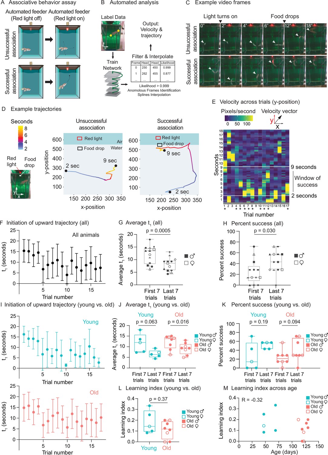
(A) Schematic for the killifish positive associative behavior assay. The red light switches on at 2 s after the video recording starts, and the food is dropped at the water surface 7 s later (so 9 s after the recording starts). Unsuccessful association occurs when the killifish does not initiate a surface-bound trajectory within the 7 s window, between the light turning on and the food dropping (so between 2 and 9 s after the recording starts) (top row). Successful association occurs when the killifish initiates a surface-bound trajectory within this 7 s window (bottom row). (B) Schematic for the automated analysis pipeline. The head and tail positions of the fish and the location of where food was dropped were annotated for selected frames and used to train the DeepLabCut network. After processing all the videos on the trained settings, the results were filtered based on likelihood, anomalous frames were identified and removed, and splines interpolation was performed (see ‘Materials and methods’). The resulting head positions of the fish were used for velocity and trajectory calculations. (C) Recording video frames from the front of the 2.8 L tank. Top row, an example trial (trial 4) of fish 3, where this fish was unsuccessful in associating food with the red light. Bottom row, an example trial (trial 17) where this fish was successful in associating food with light by moving toward the water surface after the red light turns on and before food is dropped. White arrow points to the fish’s position. From the front of the tank, a 2.8 L tank is approximately 14 cm tall and 10 cm wide. (D) Trajectory traces generated by the automated pipeline for the videos in (C). The x-positions (along the tank width) and y-positions (along the tank height) of fish 3 were tracked at each video frame from 2 s after the recording started to 9 s, and colored according to time. The food drop site indicates where the food arrives at the water surface, and the red light, where the LED light is located. Trial 4, a trial of unsuccessful association; trial 17, a trial of successful association. Sec, seconds. (E) The vertical component (y-component) of the fish’s (fish 3) velocity, graphed as a heatmap across trial number. The rolling average of 20 frames is plotted for each second of each trial. When the fish exhibits a fast trajectory toward the surface, the pixels/s value is higher (more yellow); whereas when the fish exhibits a slow trajectory toward the surface (or away from surface), the pixels/s value is smaller (bluer). Asterisks indicate successful trials. (F) The initiation time of the first surface-bound trajectory (t1) across trials for all fish, quantified by the automated pipeline. Each fish went through 17 trials. The mean t1 for all the fish was calculated for each trial (n = 13), then plotted as a function of trial numbers. A trial was considered successful if t1 was between 2 and 9 s (inclusive). Error bars represent 1 standard deviation above and below the mean t1. (G) The average t1 of the first seven trials vs. the last seven trials for each fish, quantified by the automated pipeline. Each symbol represents the average t1 for one fish, and the same symbol denotes the same fish. Males, closed symbols; females, open symbols. Significance determined by a two-tailed Wilcoxon matched-pairs signed-rank test, where the average t1 from the first and last seven trials of the same fish is a matched pair. (H) The percentage of successful trials for the first seven trials vs. the last seven trials of each fish, quantified by the automated pipeline. The symbols’ shape and color, and the statistics are the same as in (G). (I) The initiation time of the first surface-bound movement (t1) across trials for young vs. old fish, quantified by the automated pipeline and graphed as in (F). Young, blue; old, red. (J) The average t1 of the first seven trials vs. the last seven trials, for young (blue) or old (red) fish, quantified by the automated pipeline. Males, closed symbols; females, open symbols. Statistics are the same as in (G). (K) The percentage of successful trials for the first seven trials vs. the last seven trials, for young (blue) or old (red) fish, quantified by the automated pipeline. Males, closed symbols; females, open symbols. Statistics are the same as in (G). (L) Learning index for young (blue) and old (red) killifish, quantified by the automated pipeline. The learning index is defined as the inverse of the first trial number for an animal to achieve two consecutive successes. Males, closed symbols; females, open symbols. Significance determined using a two-tailed Wilcoxon rank-sum test. (M) Learning index plotted as a function of the fish’s age, quantified by the automated pipeline. Males, closed symbols; females, open symbols. R, Pearson correlation coefficient.
-
Figure 6—source data 1
Experimental metadata for behavior experiments.
- https://cdn.elifesciences.org/articles/69008/elife-69008-fig6-data1-v2.xlsx
-
Figure 6—source data 2
Unfiltered raw trajectory data output from DeepLabCut.
- https://cdn.elifesciences.org/articles/69008/elife-69008-fig6-data2-v2.zip
-
Figure 6—source data 3
Filtered and interpolated trajectory data with velocity calculations.
- https://cdn.elifesciences.org/articles/69008/elife-69008-fig6-data3-v2.zip
-
Figure 6—source data 4
Initiation of upward trajectory value (t1) summary for automatic quantification.
- https://cdn.elifesciences.org/articles/69008/elife-69008-fig6-data4-v2.xlsx
-
Figure 6—source data 5
Fish angular coordinate data for compass plots.
- https://cdn.elifesciences.org/articles/69008/elife-69008-fig6-data5-v2.zip
-
Figure 6—source data 6
Initiation of upward trajectory value (t1) summary for manual quantification.
- https://cdn.elifesciences.org/articles/69008/elife-69008-fig6-data6-v2.xlsx
-
Figure 6—source data 7
Manual quantification of behavior for female killifish.
- https://cdn.elifesciences.org/articles/69008/elife-69008-fig6-data7-v2.xlsx
-
Figure 6—source data 8
Manual quantification of behavior for male killifish.
- https://cdn.elifesciences.org/articles/69008/elife-69008-fig6-data8-v2.xlsx
Figure 6—figure supplement 1
Use of automated feeder for assessing positive associative learning behavior.
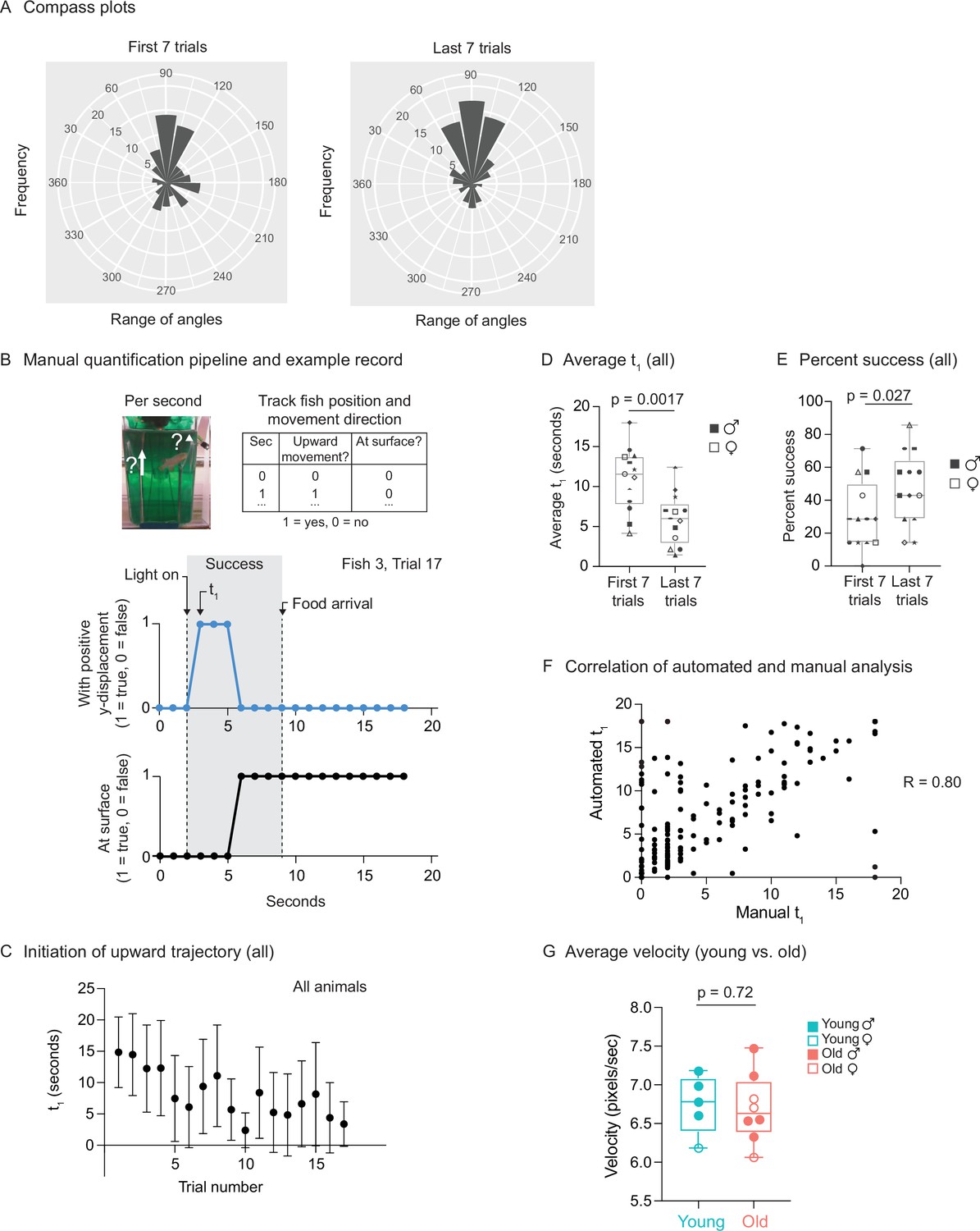
(A) Compass plots for the first seven trials or last seven trials, representing the frequency distribution of the angles of movement, for all fish, between the light turning on (at 2 s) and the food dropping (at 9 s). For each fish, the initial position (at 2 s) and the final position (at 9 s) were converted from Cartesian coordinates (x, y) to polar coordinates (r, θ), and the angular coordinate (θ) of the vector (from the initial position to the final position) was converted from radians to degrees. The angular coordinates (θ) from all the fish from multiple trials (the first seven trials or the last seven trials) were binned (bin size = 20°). The frequency distribution (histograms centered on the midpoint of each bin) is plotted. An angular coordinate of 90° would indicate that the average movement of the fish between 2 and 9 s was directly to the surface. Each ‘wedge’ on the compass plot represents a bin. The wedge is directed toward the angle (out of 360°) that represents the midpoint of the bin and has a radius that indicates the frequency of angles in the bin (larger radius indicating that more velocity vectors fallen into that bin). All the bins have the same origin. (B) Schematic for the manual analysis pipeline. Top, schematic for quantification metrics. For each trial, the fish position and movement were tracked second by second. If the fish displays any positive y-axis displacement (tracked by the midpoint of the fish) at a given second, then a score of ‘1’ would be given to metric 1 (‘upward movement’). If the fish is located within ~0.5 cm from the water surface, then a score of ‘1’ would be given to metric 2 (‘at surface‘). Middle, occurrence of positive y-displacement; bottom, presence of the fish at the water surface, across the 18 s for trial 17 of fish 3. Light turns at 2 s after the video recording starts, and the food drops at the water surface at 9 s. The initiation time of the first surface-bound trajectory (t1) is at 3 s, which is between 2 and 9 s. Thus, this trial is considered ‘successful.’ (C) The initiation time of the first surface-bound trajectory (t1) across trials for all fish, quantified manually. The mean t1 and error bars are plotted as in Figure 6F. (D) The average t1 for the first seven trials vs. the last seven trials, quantified manually. The symbols’ shape and color, and the statistics are the same as in Figure 6G. (E) The percentage of successful trials for the first seven trials vs. the last seven trials, quantified manually. The symbols’ shape and color, and the statistics are the same as in Figure 6G. (F) Correlation of t1 between the automated and manual pipelines. Each point represents a trial, with t1 quantified manually (‘manual t1’) or using the automated pipeline (‘automated t1’). A total of 219 trials were quantified, with all the trials from the 13 fish pooled. R, Pearson correlation. (G) The average velocities for young and old fish, quantified by the automatic pipeline. For each fish, the 20-frame rolling average velocities were averaged across all frames and all trials. Each dot represents the trial average of one fish. Males, closed symbols; females, open symbols. Significance determined by Wilcoxon rank-sum test.
Figure 6—video 1
Example of a trial with a ‘successful’ association (trial 17, fish 3).
Figure 6—video 2
Example of a trial with an ‘unsuccessful’ association (trial 4, fish 3).
Tables
Table 1
Automated feeding allows for more flexible, frequent, and precise feedings than manual feeding.
Manual feeding is restricted to the times of the day when researchers can enter the animal facilities based on day/night cycles, whereas automated feeding can be programmed to occur at any time of the day or night. Manual feeding is restricted by the researcher’s ability to feed, while automated feeding can occur as frequently as 144 times per day. Manual feeding requires individual attention to each tank on a daily basis, multiple times per day, whereas automated feeding requires an initial setup and biweekly checks to replace batteries and add food to the devices. Manual feeding is relatively imprecise at 0.016 (the inverse of the variance of food delivered), while automated feeding has a higher precision at 0.512.
| Manual feeding | Automated feeding | |
|---|---|---|
| Schedule flexibility | Limited to weekday working hours | 24/7 |
| Maximum frequency | 2–3 times a day | 144 times a day |
| Labor required | Daily, linearly increasing with tanks | Initial setup and biweekly checks |
| Precision | Low, with batch effects for different individuals (0.016) | Higher (0.512) |
Additional files
Download links
A two-part list of links to download the article, or parts of the article, in various formats.
Downloads (link to download the article as PDF)
Open citations (links to open the citations from this article in various online reference manager services)
Cite this article (links to download the citations from this article in formats compatible with various reference manager tools)
An automated feeding system for the African killifish reveals the impact of diet on lifespan and allows scalable assessment of associative learning
eLife 11:e69008.
https://doi.org/10.7554/eLife.69008


