Mimicry can drive convergence in structural and light transmission features of transparent wings in Lepidoptera
- Institut de Systématique, Evolution, Biodiversité (ISYEB), CNRS, Muséum national d'Histoire naturelle, Sorbonne Université, EPHE, Université des Antilles, France
- Centre de Recherche sur la Conservation (CRC), CNRS, MNHN, Ministère de la Culture, France
- Institut de Physique du Globe de Paris (IPGP), Université de Paris, CNRS, France
- Institut des NanoSciences de Paris (INSP), Sorbonne Université, CNRS, France
- Marine Biological Laboratory, United States
- Department Integrative Biology, University of California Berkeley, United States
- Centre d'Ecologie Fonctionnelle et Evolutive (CEFE), CNRS, Univ Montpellier, France
Figures
Figure 1 with 3 supplements

Test of convergence of transmission properties between co-mimetic species.
Figure 1—figure supplement 1
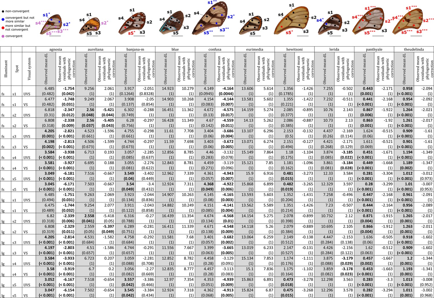
Results of the test of convergence of achromatic (dL) contrasts for each mimicry ring.
All the visual systems (VS and UVS) and the illuminants (large gap ‘lg’ and forest shade ‘fs’) tested are presented. For each spot measured on the forewing and for each mimicry ring (see figure on top of the table), the mean achromatic contrast has been compared to what is expected at random (1st column highlighted in grey for each mimicry ring, p-value corrected for multiple testing with ‘Holm’ method in brackets) and to what is expected according to the phylogeny (2nd column for each mimicry ring, p-value corrected for multiple testing with ‘Holm’ method in brackets). Mean achromatic contrasts statistically different from what is expected at random or given the phylogeny are highlighted in bold. To test whether mean achromatic contrast between co-mimetic species of a given mimicry ring is smaller to what is expected at random, we randomised the value of the achromatic contrast 10,000 times over each pair of species, we calculated the mean achromatic contrast for these co-mimetic species for each randomisation and we calculated the p-value as the proportion of randomisations where the mean achromatic contrast for co-mimics is smaller than the observed mean achromatic contrast. To test whether the mean achromatic contrast between co-mimetic species of a given mimicry ring is smaller than what might be expected given their phylogenetic relationship, we did a linear model between achromatic contrasts and phylogenetic distances to account for the effect of phylogeny on the achromatic contrast and we considered the mean of residuals for co-mimetic species of a given mimicry ring. If co-mimetic species are more similar than expected according to the phylogeny, the mean of residuals should be negative. To test whether the mean of residuals is smaller than expected according to the phylogeny, we randomised residuals over all pair of species and we calculated the mean of residuals for co-mimetic species of a given mimicry ring. We calculated ‘p-value with phylogenetic correction’ as the proportion of randomisations where the mean of residuals is smaller than the observed mean of residuals. Each spot measured is localised on the forewing and the results of the test are represented by the colour of the spot. Black spots stand for spots that are neither more similar than expected at random nor convergent (more similar when phylogenetic relationships are accounted for) between co-mimetic species. Blue spots stand for spots that are not more similar than expected at random but which are convergent because they are more similar that what might be expected according to their phylogenetic distance. Red spots stand for spots that are more similar than expected at random but not convergent. Purple spots stand for spots that are both more similar than expected at random and convergent (more similar than what might be expected based on phylogenetic distance). Tests’ p-values corrected for multiple testing with the ‘Holm’ method are represented with the following symbols: ‘***’ p < 0.001, ‘**’ p < 0.01, ‘*’ p < 0.05.
Figure 1—figure supplement 2
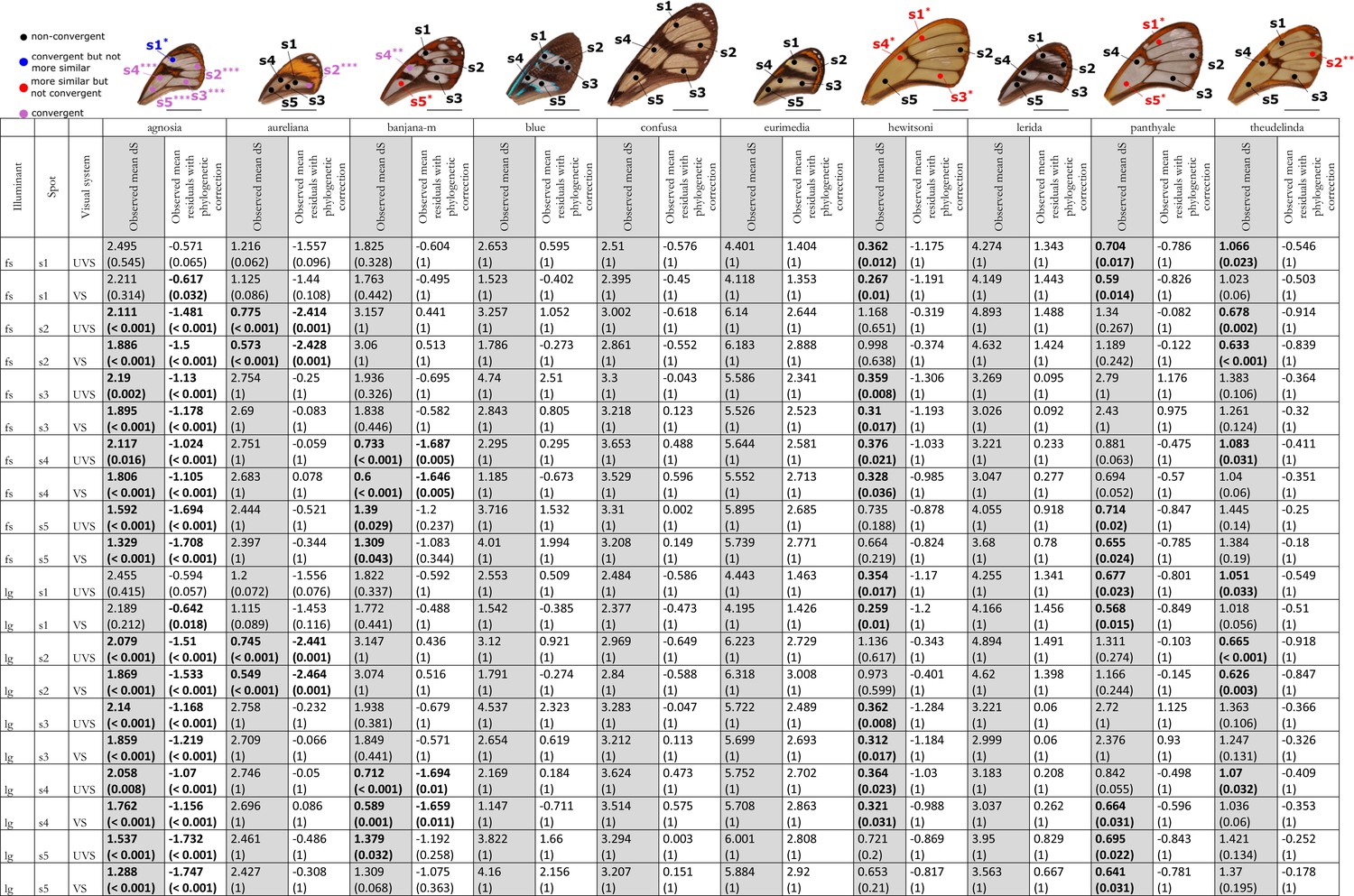
Results of the test of convergence of chromatic (dS) contrasts for each mimicry ring.
All the visual systems (VS and UVS) and the illuminants (large gap ‘lg’ and forest shade ‘fs’) tested are presented. For each spot measured on the forewing and for each mimicry ring (see figure on top of the table), the mean chromatic contrast has been compared to what is expected at random (1st column highlighted in grey for each mimicry ring, p-value corrected for multiple testing with ‘Holm’ method in brackets) and to what is expected according to the phylogeny (2nd column for each mimicry ring, p-value corrected for multiple testing with ‘Holm’ method in brackets). Mean chromatic contrasts statistically different from what is expected at random or given the phylogeny are highlighted in bold. To test whether mean chromatic contrast between co-mimetic species of a given mimicry ring is smaller to what is expected at random, we randomised the value of the chromatic contrast 10,000 times over each pair of species, we calculated the mean chromatic contrast for these co-mimetic species for each randomisation and we calculated the p-value as the proportion of randomisations where the mean chromatic contrast for co-mimics is smaller than the observed mean chromatic contrast. To test whether the mean chromatic contrast between co-mimetic species of a given mimicry ring is smaller than what might be expected given their phylogenetic relationship, we did a linear model between chromatic contrasts and phylogenetic distances to account for the effect of phylogeny on the chromatic contrast and we considered the mean of residuals for co-mimetic species of a given mimicry ring. If co-mimetic species are more similar than expected according to the phylogeny, the mean of residuals should be negative. To test whether the mean of residuals is smaller than expected according to the phylogeny, we randomised residuals over all pair of species and we calculated the mean of residuals for co-mimetic species of a given mimicry ring. We calculated ‘p-value with phylogenetic correction’ as the proportion of randomisations where the mean of residuals is smaller than the observed mean of residuals. Each spot measured is localised on the forewing and the results of the test are represented by the colour of the spot. Black spots stand for spots that are neither more similar than expected at random nor convergent (more similar when phylogenetic relationships are accounted for) between co-mimetic species. Blue spots stand for spots that are not more similar than expected at random but which are convergent because they are more similar that what might be expected according to their phylogenetic distance. Red spots stand for spots that are more similar than expected at random but not convergent. Purple spots stand for spots that are both more similar than expected at random and convergent (more similar than what might be expected based on phylogenetic distance). Tests’ p-values are represented with the following symbols: ‘***’ p < 0.001, ‘**’ p < 0.01, ‘*’ p < 0.05.
Figure 1—figure supplement 3
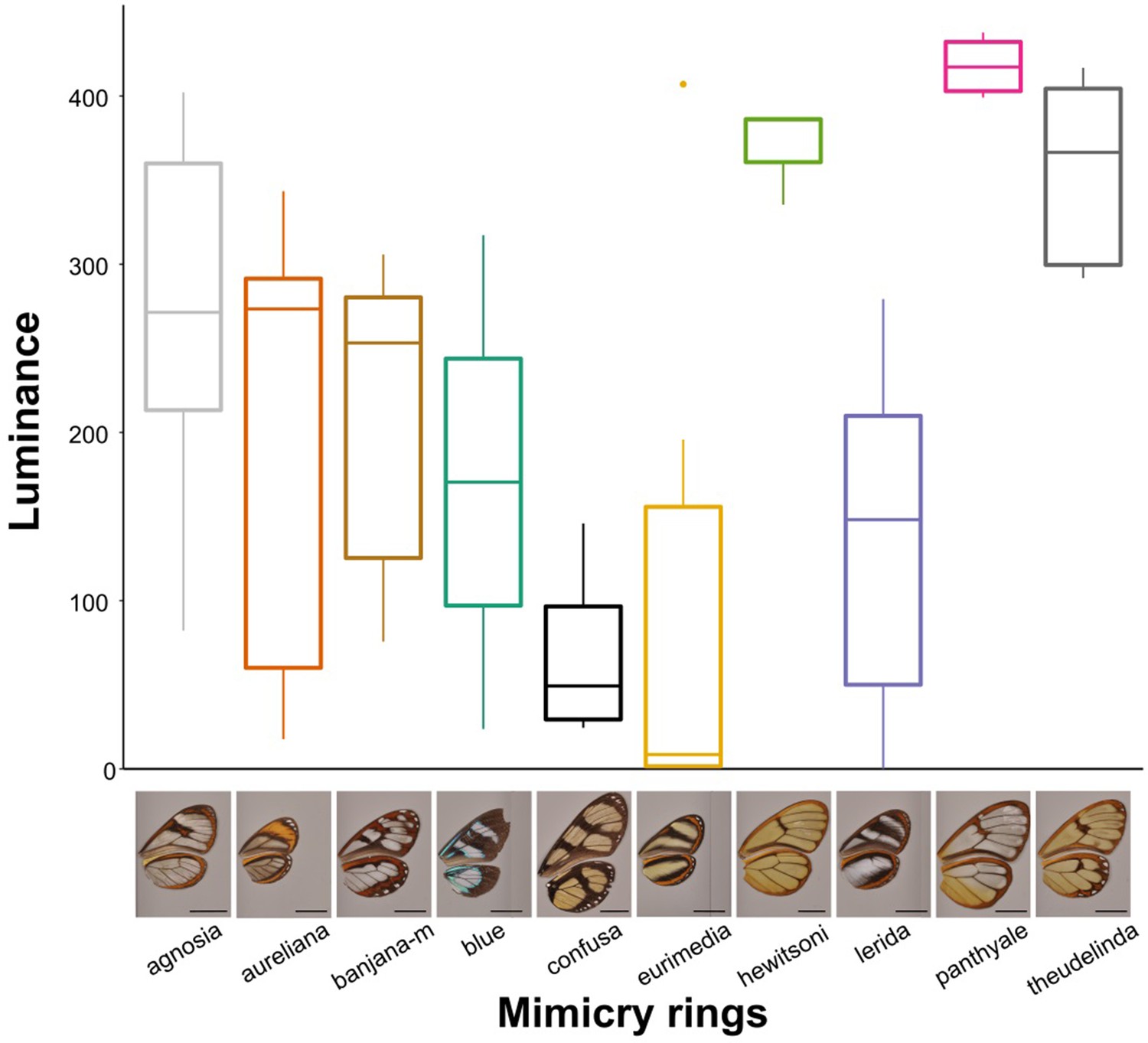
Differences in an avian analogue of luminance (quantum catch for brightness channel) between mimicry rings.
The values presented here correspond to a vision model for large gap illuminants and UVS visual system, for the most proximal spot on the forewing. Results for other spots, other visual systems and illuminants are similar.
Figure 2
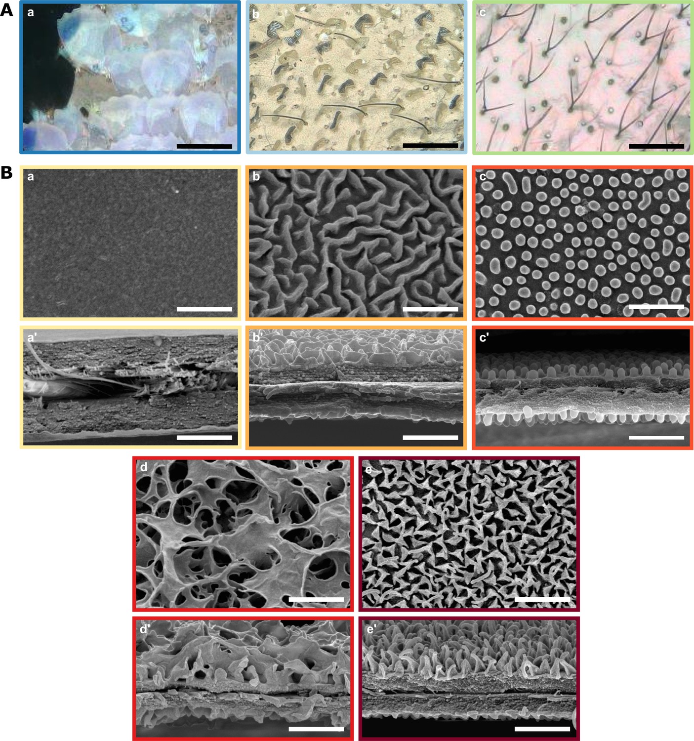
Diversity of micro- and nanostructures involved in transparency.
(A) Diversity of microstructures. (a) transparent lamellar scales of Hypocrita strigifera, (b). erected lamellar scales of Methona curvifascia and (c). piliform scales of Hypomenitis ortygia. Scale bars represent 100 µm. (B) Diversity of nanostructures. (a), (b), (c), (d) and (e) represent top views and (a’), (b’), (c’), (d’), and (e’) represent cross section of wing membrane. Scale bars represent 1 µm. (a), (a’). absence of nanostructure in Methona curvifascia; (b), (b’). maze nanostructures of Megoleria orestilla; (c), (c’). nipple nanostructures of Ithomiola floralis; (d), (d’). sponge-like nanostructures of Oleria onega; (e), (e’). pillar nanostructures of Hypomenitis enigma. Each coloured frame corresponds to a scale type or nanostructure type, as defined in Figure 3.
Figure 3 with 1 supplement
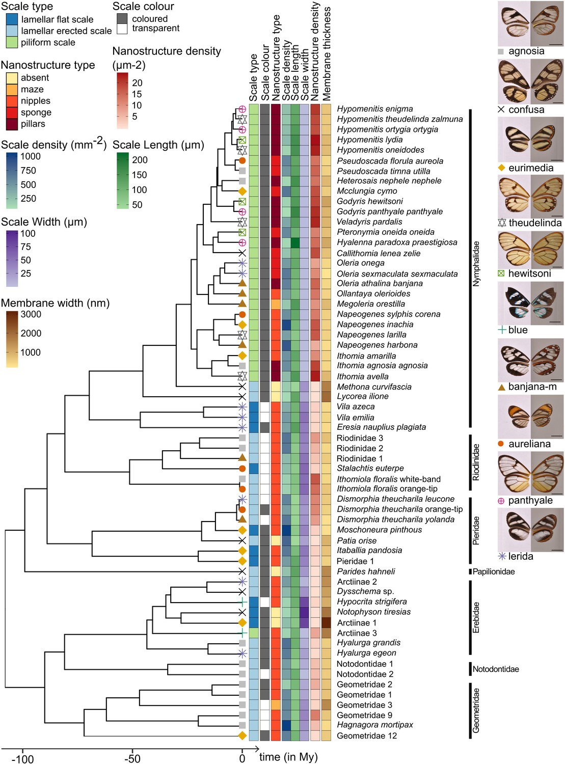
Phylogeny of the 62 species considered in this study and distribution of traits along the phylogeny.
Mimicry rings are represented by a symbol and a specimen is given as an example for each mimicry ring. Dorsal side of wings has been photographed on a white background (left column) and ventral side on a gray background to highlight the transparent patches (right column). The x axis represents time in million years (My).
Figure 3—figure supplement 1
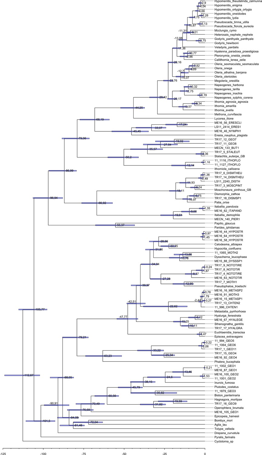
Maximum clade credibility tree of all the specimens obtained with BEAST 1.8.3.
Each tip label represents one individual and the species name, when known, is given in the Supplementary file 2a. Median node age is given at each node and the 95 % interval of the node age post distribution is represented by a horizontal blue bar.
Figure 4 with 1 supplement
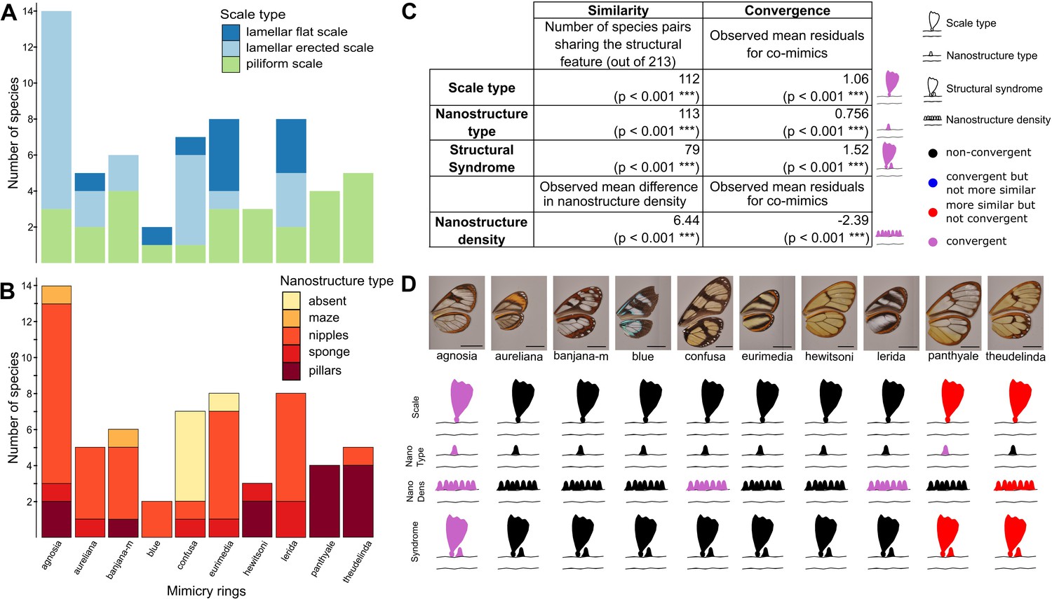
Convergence of structures underlying transparency.
(A,B) Distribution of micro- (A) and nanostructures (B) among the different mimicry rings (indicated at the bottom on panel B). (C) Results of the test of convergence for structural features (either scale type, nanostructure type, nanostructure density or structural syndrome, that is, the association of scale type and nanostructure type). To test for similarity independently of the underlying process, we assessed whether the number of co-mimetic species sharing the same structural feature (out of 213 co-mimetic species pairs) was higher than expected at random or whether difference in nanostructure density was smaller than expected at random. To do so, we randomised 10,000 times the sharing variable (or difference in nanostructure density) over all pairs of species and we calculate the p-value (indicated in brackets, corrected for multiple testing with the ‘Holm’ method) as the proportion of randomisations where the number of co-mimetic species sharing the structural feature is higher than the observed number of co-mimetic species pairs sharing the structural feature (or where the mean difference in nanostructure density is smaller than the observed mean difference in nanostructure density). To test for convergence on structural features, we tested whether the observed mean residuals of the generalised linear model linking structure sharing and phylogenetic distance was higher than expected given the phylogeny (or whether mean residuals of the linear model linking difference in nanostructure density and phylogenetic distance was smaller than expected given the phylogeny) and we calculated the p-value (indicated in brackets, corrected for multiple testing with the ‘Holm’ method) as the proportion of randomisations of model’s residuals where the mean residuals for co-mimetic species is higher (or smaller for nanostructure density) than the observed mean residuals for co-mimetic species. (D) Graphical representation of the results of the test of convergence for each mimicry ring. For each mimicry ring, we tested whether the structural features were more similar than expected at random and given the phylogeny (with the same tests described above, see Figure 4—figure supplement 1 for details). We represented the results for scale type, nanostructure type, nanostructure density and structural syndrome. Black structures indicate neither more similar structures than expected at random nor convergent structures; red structures indicate structure more similar than expected at random but not convergence; blue structures indicate structures not more similar than expected at random but convergent and purple structures indicate convergent structures.
Figure 4—figure supplement 1
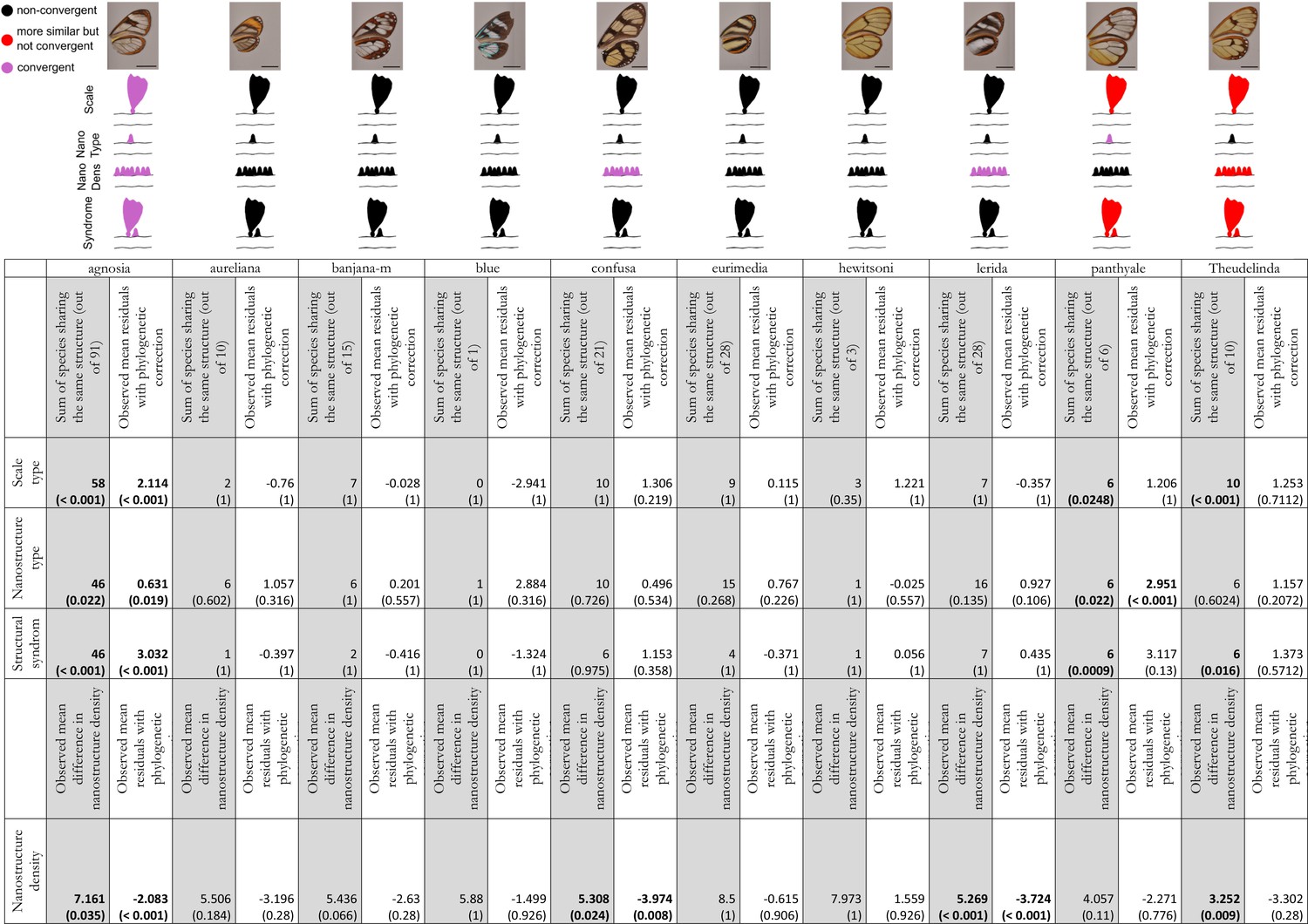
Results of the test of convergence of structural features for each mimicry ring.
We consider convergence in scale type (either piliform scale, lamellar erected scale or lamellar flat scale), in nanostructure type (either absent, maze, nipples, sponge or pillars), in nanostructure density and in structural syndrome which corresponds to the association of one type of scales with one type of nanostructures. For each mimicry ring, we tested the similarity of structures between co-mimetic species, independently of their phylogenetic relationship by comparing the sum of co-mimetic species sharing the same structure or the mean difference in nanostructure density to what is expected at random (1st column, highlighted in grey for each mimicry ring; we specified the number of co-mimetic species pair in brackets for each mimicry ring), based on 10,000 randomisations of the variable ‘shared structures’. The p-value (in brackets, here corrected for multiple testing with ‘Holm’ method) has been calculated as the proportion of randomisations where the sum of co-mimetic species sharing the same structure is higher than the observed sum of co-mimetic species sharing the same structure. We also tested the putative convergence of structures between co-mimetic species by performing a generalised linear model with binomial error linking the variable ‘shared structures’ (one if the co-mimetic species share the same structures, 0 otherwise) and phylogenetic distance or a linear model linking difference in nanostructure density and phylogenetic distance. We compared the mean of the model residuals for co-mimetic species to what is expected according to the phylogeny (2nd column for each mimicry ring), based on 10,000 randomisations of residuals along all pairs of species. The p-value (in brackets, here corrected for multiple testing with ‘Holm’ method) was calculated as the proportion of randomisations where the mean of residuals is higher than the observed mean of residuals. The results are presented graphically in the figure above the table. Black structures indicate neither more similar than expected at random nor convergent structures; red structures indicate structures more similar than expected at random but not convergent and purple structures indicate both more similar than expected at random and convergent structures.
Figure 5 with 1 supplement
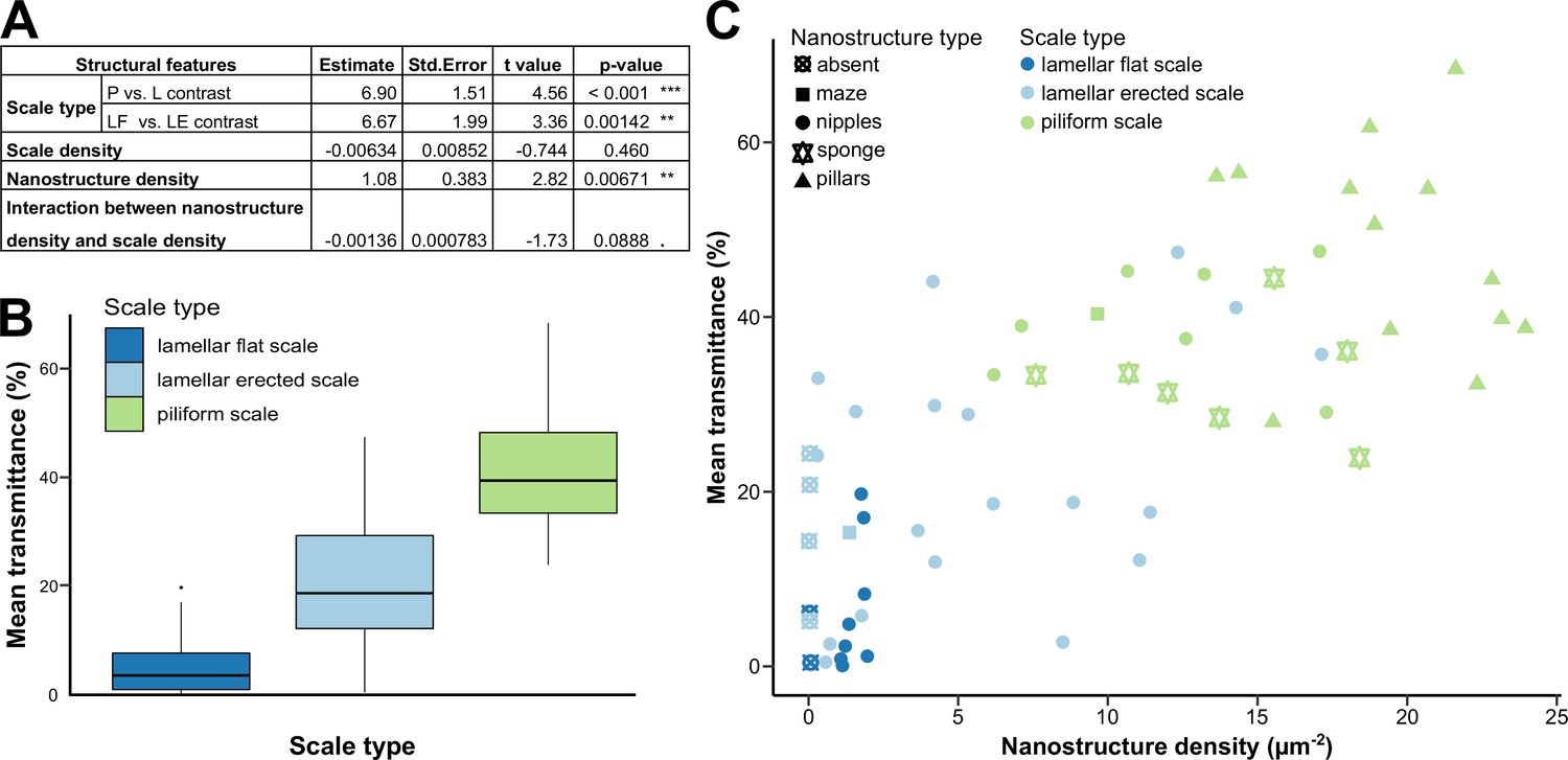
Link between mean transmittance over 300–700 nm and structural features.
(A) Results of the best PGLS model (F5,56 = 26.65 (p-value < 0.001 ***), AICc = 469.9, Radj2 = 0.678, λ = 0 (p-value < 0.001 ***)) linking mean transmittance and micro- and nanostructure features. The explicative variables have not been scaled or centred. Nanostructure density has been measured in µm–2 and scale density in mm–2. Scale type is a categorical variable with three levels either lamellar flat scale (LF), lamellar erected scale (LE) or piliform scale (P). (B) Link between mean transmittance measured between 300 and 700 nm and scale type. (C) Link between mean transmittance measured between 300 and 700 nm and nanostructure density, nanostructure type (represented by different shapes) and scale type (represented by different colours). NB. We considered the spot corresponding to the location of the SEM images for mean transmittance.
-
Figure 5—source data 1
Raw transmittance spectra presented by mimicry ring and for each species.
For each specimen, the smoothed spectra corresponding to the five spots measured with different colours are shown. Species are grouped by mimicry ring, presented in alphabetical order. The following species are considered as opaque macroscopically: · ‘agnosia’ mimicry ring: Hagnagora mortipax; · ‘aureliana’ mimicry ring: Stalachtis euterpe; · ‘banjana-m’ mimicry ring: Riodin_1; · ‘blue’ mimicry ring: Hypocrita strigifera; · ‘eurimedia’ mimicry ring: Arctiinae1, Geo12, Moschoneura pinthous, Itaballia pandosia, Pieridae1; · ‘lerida’ mimicry ring: Vila emilia, Eresia nauplius plagiata.
- https://cdn.elifesciences.org/articles/69080/elife-69080-fig5-data1-v2.pdf
Figure 5—figure supplement 1
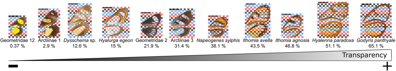
Gradient of transparency among the studied species as illustrated by 11 species.
Specimens are ordered from the least to the most transparent: average mean transmittance over the five spots measured is presented in percentage under each species name. The ventral side of their wings is presented on a checkered background to clearly see the transparent areas. The scalebar in the top left of each photo represents 1 cm.
Author response image 1
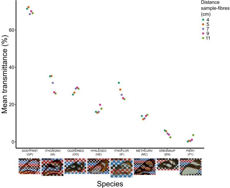
Effect of distance between fibres and wing sample on mean transmittance for each species (normal incidence: 0°).
Each point represents the measurement of mean transmittance for an incident angle of 0 degree (which corresponds to our original setting) and a distance between fibres and sample ranging from 4 to 11 cm. A photo of the forewing against a chequered background is presented below the graph and the scale bar represent 1 cm.
Author response image 2
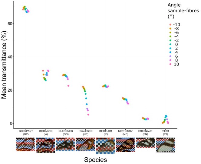
Effect of incident angle between fibres and wing sample for each species considered at a distance of 11 cm (which corresponds to the original setting).
Each point represents the measurement of mean transmittance at a distance of 11 cm between fibres and sample and at an incident angle ranging from -10° to 10°. A photo of the forewing against a chequered is presented below the graph and the scale bar represent 1 cm.
Tables
Author response table 2
Results of the linear model linking mean transmittance (B2) with species, distance and incident angle between fibres and the wing sample and the interaction between incident angle and distance (F10, 429 = 2691, p-value < 0.001, R2adj = 0.984).
Species are represented by their initials (GP: Godyris panthyale, IA: Ithomia agnosia, OO: Oleria onega, EN: Eresia nauplius, HE: Hyalurga egeon, IF: Ithomiola floralis, MC: Methona curvifascia, PIER1: Pieridae 1). The p-values presented are equal to the p-value of the mixed model adjusted for type III sums of squares.
| Variable | Estimate(mean ± sd) | t-value | p-value | |
|---|---|---|---|---|
| Intercept | 25.43 ± 0.38 | 67.0 | < 2*10-16 *** | |
| Species | Piliform coloured scales>Lamellar scales(GP, IA, OO) > (EN, HE, IF, MC, P1) | 3.89 ± 0.03 | 122.3 | < 2*10-16 *** |
| Within Lamellar scales:Lamellar erect scales > lamellar flat scales(HE, IF, MC) > (EN, P1) | 3.10 ± 0.06 | 48.7 | < 2*10-16 *** | |
| Within lamellar erect scales: transparent scales> coloured scales(IF) > (HE, MC) | 3.80 ± 0.14 | 26.7 | < 2*10-16 *** | |
| Within piliform coloured scales:pillars nanostructures > sponge nanostructures(GP, IA) > (OO) | 7.94 ± 0.14 | 55.7 | < 2*10-16 *** | |
| Within lamellar erect coloured scales, nipples nanostructures > absent nanostructure(HE) > (MC) | 1.19 ± 0.25 | 4.8 | 2.1*10-6 *** | |
| Within piliform coloured scales:Ring panthyale > ring agnosia(GP) > (IA) | 18.55 ± 0.25 | 75.2 | < 2*10-16 *** | |
| Within opaque species:Ring lerida>ring eurimedia(EN) > (P1) | -1.52 ± 0.25 | 6.18 | 1.5*10-9 *** | |
| Distance between fibres and sample | -0.0231 ± 0.005 | -4.81 | 2.09*10-6 *** | |
| Incident angle between fibres and sample | 0.056 ± 0.060 | 0.943 | 0.346 | |
| Interaction between distance and incident angle | -0.0017 ± 0.00076 | -2.36 | 0.019 * |
Author response table 1
| Appearance | Species | Abbre-viation | Mimicry ring | Microstructure |
|---|---|---|---|---|
| Highly transparent | Godyris panthyale | GP | panthyale | piliform coloured scales |
| Ithomia agnosia | IA | agnosia | piliform coloured scales | |
| Slightly scattering | Oleria onega | OO | lerida | piliform coloured scales |
| Hyalurga egeon | HE | lerida | lamellar erect coloured scales | |
| Moderately transparent | Methona curvifascia | MC | confusa | lamellar erect coloured scales |
| Ithomiola floralis | IF | agnosia | lamellar erected transparent scales | |
| Opaque | Pieridae1 | P1 | eurimedia | lamellar flat coloured scales |
| Eresia nauplius plagiata | EN | lerida | lamellar flat coloured scales |
Additional files
-
Supplementary file 1
Supplementary files related to transparent wing optical properties and structures.
(a) Tests of convergence of transparent patches, as perceived by predators, among co-mimetic species: achromatic contrasts. All the visual systems (VS and UVS) and the illuminants (large gap ‘lg’ and forest shade ‘fs’) tested are presented. We tested whether mean achromatic contrast (dL) between co-mimetic species is smaller than expected at random (expected mean dL for co-mimics ± standard deviation (sd)). To do so, we randomised the value of the achromatic contrast 10,000 times over each pair of species and we calculated the p-value as the proportion of randomisations where the mean achromatic contrast for co-mimics is smaller than the observed mean achromatic contrast. We also considered whether co-mimetic species were more similar than expected according to their phylogenetic relationship. To do so, we did a linear model between achromatic contrasts and phylogenetic distances to account for the effect of phylogeny on the achromatic contrast and we considered the mean of residuals for co-mimetic species. If co-mimetic species are more similar than expected according to their phylogenetic relationship, the mean of residuals should be negative. To test whether the mean of residuals is smaller than expected according to the phylogeny, we randomised residuals over all pair of species and we calculated the mean of residuals for co-mimetic species. We calculated ‘p-value with phylogenetic correction’ as the proportion of randomisations where the mean of residuals is smaller than the observed mean of residuals. If the p-value is smaller than 0.05, it means that co-mimetic species are more similar than expected at random and if the p-value with phylogenetic correction is smaller than 0.05, it means that the observed similarity is due to convergence. We also present p-values corrected with multiple testing with the ‘Holm’ method.
(b) Tests of convergence of transparent patches, as perceived by predators, among co-mimetic species: chromatic contrasts. All the visual systems (VS and UVS) and the illuminants (large gap ‘lg’ and forest shade ‘fs’) tested are presented. We tested whether mean chromatic contrast (dS) between co-mimetic species is smaller than expected at random (expected mean dS for co-mimics ± standard deviation (sd)). To do so, we randomised the value of the chromatic contrast 10,000 times over each pair of species and we calculated the p-value as the proportion of randomisations where the mean chromatic contrast for co-mimics is smaller than the observed mean chromatic contrast. We also considered whether co-mimetic species were more similar than expected according to their phylogenetic relationship. To do so, we did a linear model between chromatic contrasts and phylogenetic distances to account for the effect of phylogeny on the chromatic contrast and we considered the mean of residuals for co-mimetic species. If co-mimetic species are more similar than expected according to their phylogenetic relationship, the mean of residuals should be negative. To test whether the mean of residuals is smaller than expected according to the phylogeny, we randomised residuals over all pair of species and we calculated the mean of residuals for co-mimetic species. We calculated ‘p-value with phylogenetic correction’ as the proportion of randomisations where the mean of residuals is smaller than the observed mean of residuals. If the p-value is smaller than 0.05, it means that co-mimetic species are more similar than expected at random and if the p-value with phylogenetic correction is smaller than 0.05, it means that the observed similarity is due to convergence. We also presented p-values corrected with multiple testing with the ‘Holm’ method.
(c) Phylogenetic signal for structural features and transmission properties. Measure of the phylogenetic signal (estimated as Pagel’s λ and Blomberg’s K for quantitative traits; δ for multicategorial traits and Purvis and Fritz’s D for binary traits) of the different features associated to micro- and nanostructures and of mean transmittance. When λ or K are equal to 0, the trait is distributed randomly across the phylogeny, whereas when λ or K are equal to one the trait evolves according to a Brownian motion model along the phylogeny. When D is equal to 1, the trait is randomly distributed across the phylogeny whereas when D is equal to 0, the trait evolves according to Brownian motion model along the phylogeny. The value of δ can be any positive real number and the higher this value, the higher the phylogenetic signal of the trait. For δ, to determine whether the distribution of the trait is different from a random distribution we randomised the trait 1000 times along the phylogeny, and we calculated δ for each randomisation. We then compared the value of δ to the distribution of values of δ under the random hypothesis and we calculated a p-value as the number of randomisations in which δ is higher than the value obtained for the real distribution of the trait.
(d) Information about specimens used for optical and structural measurements.
(e) Results of the eight best PGLS (Phylogenetic Generalised Least Square) models (AICc within an interval of 2 of that of the best model). For each model, we give: the F statistic with the degrees of freedom in indices, the p-value of the model (in brackets), the corrected Akaike criterion (AICc) of the model, the adjusted R² and the value of lambda branch length transformation which has been estimated by maximum likelihood given the statistical model linking traits. When λ equals 1, the branch length of the phylogeny is unchanged, whereas when λ equals 0 branch length is set to zero, meaning that all species are considered independent. The ‘p-values’ for the value of λ, given in brackets, are the probability that λ is equal to 0 or to 1. We also give for each model the value of the coefficient estimate for each variable tested and the p-value (in brackets) is represented with the follow symbols: '***': p < 0.001; '**': p < 0.01; '*': p < 0.05; '.' : p < 0.1; 'n.s.': not significantly different from 0. NA means that the variable was not retained in the model.
(f) Technical repeatability of transmission measurements and structural features. For each grouping factor (either the number of species or the number of individuals or the total number of different spots measured; indicated in the ‘number of groups’ column), we calculated the value of repeatability R based on several measurements of the same element of a grouping factor. The calculation of repeatability is based on mixed linear models. Confidence intervals are calculated with parametric bootstraping and p-values (associated to the test R > 0) are calculated with two methods: with likelihood ratio test comparing the likelihood of the model with and without the tested random effect and with permutation tests. We also calculated the coefficient of variation (CV, as the mean of the group devided by the standard error) for each group and we give here the median value of the CV distribution.
(g) Biological repeatability of transmission measurements and structural features. For each grouping factor (either the number of species, or the number of different spots measured per species; indicated in the ‘number of groups’ column), we calculated the value of repeatability R based on several measurements of the same element of a grouping factor. The calculation of repeatability is based on mixed linear model. Confidence intervals are calculated with parametric bootstraping and p-values (associated to the test R > 0) are calculated with two methods: with likelihood ratio test comparing the likelihood of the model with and without the tested random effect and with permutation tests. We also calculated the coefficient of variation (CV, as the mean of the group devided by the standard error) for each group and we give here the median value of the CV distribution.
(h) Similarity between conspecific individuals for chromatic and achromatic contrasts. To test whether conspecific individuals were perceived as more similar than expected at random for each spot on the forewing, we randomised the contrasts over all pair of species and we calculated the mean distance for conspecific individuals. We compared the mean phenotypic distance (either chromatic or achromatic contrast) for the observed data to the distribution of mean phenotypic distance calculated for 10,000 randomisations and we calculated the p-value as the number of randomisations where mean phenotypic distance was smaller than the observed phenotypic distance. We conclude that conspecific individuals are perceived as more similar than expected at random, implying that any individual is representative of its species.
- https://cdn.elifesciences.org/articles/69080/elife-69080-supp1-v2.xlsx
-
Supplementary file 2
Supplementary files related to phylogenetic reconstruction.
(a) Information on specimens used to infer a phylogeny.
(b) Node constraints used to calibrate the phylogeny. For all constraints, we used uniform distribution priors whose bound were determined according to 95 % HSPD inferred by Kawahara et al., 2019 on their phylogeny of Lepidoptera.
(c) Results of the best partition (based on BIC) for the eight different genes obtained with Partition Finder v1.0.1, with linked branch length and greedy algorithm. For each gene, pos1, pos2 and pos3 refer to codon positions. Only the substitution models available in BEAST were tested. GTR: general time reversible (base frequencies are variable, substitution matrix is symmetrical), HKY: Hasegawa-Kishino-Yano (base frequencies are variable, there are one transition rate and one tranversion rate), TrN: Tamura-Nei (base frequencies are variable, transversion rates are equal, transition rates are variable), I: proportion of invariable sites, G: gamma distribution (rate variation among sites is gamma distributed).
- https://cdn.elifesciences.org/articles/69080/elife-69080-supp2-v2.xlsx
-
Supplementary file 3
Supplementary files related to supplementary results: link between bird perception and optical properties; link between nanostructure type and density;comparision between wing ventral and dorsal sides.
(a) Results of the linear mixed model linking mean transmittance over 300–700 nm (physical descriptor of transparency) and coordinates in tetrahedral colour space (x, y, z) and luminance extracted from the vision model with UVS visual system and large gap ambient light (biologically relevant descriptors of transparency). For each species, the five measurements were used, and the specimen was taken as random effect, and all the variables were centred and scaled.
(b) Analysis of deviance table to check the importance of the effect of each variable on mean transmittance over 300–700 nm.
(c) Results of the PGLS model (F4,57 = 3728 (p-value < 0.001 ***), AICc = –159.4, Radj2 = 0.9959, λ = 0 (probability(λ=1) < 0.001)) linking average mean transmittance over 300–700 nm (physical descriptor of transparency) with average coordinates in tetrahedral space (x, y and z) and luminance extracted from vision models (biologically relevant descriptors of transparency).
(d) Results of the phylogenetic ANOVA on nanostructure density with nanostructure type as factor. The p-value is based on simulations.
(e) Results of the post-hoc tests (t values) to determine which type of nanostructures is different in density to others. p-values were corrected with Bonferroni correction and are indicated in brackets after t-values. Significant differences between nanostructure types are highlighted in bold.
(f) Results of the type III analysis of variance on the model linking scale density with species and side (ventral or dorsal) to determine the effect of each variable on scale density.
(g) Results of the type III analysis of variance on the model linking scale length with species, side (ventral or dorsal) and scale type (lamellar, piliform bifid or piliform monofid) to determine the effect of each variable on scale length.
(h) Results of the type III analysis of variance on the model linking scale width with species, side (ventral or dorsal) and scale type (lamellar, piliform bifid or piliform monofid) to determine the effect of each variable on scale width.
- https://cdn.elifesciences.org/articles/69080/elife-69080-supp3-v2.xlsx
-
Transparent reporting form
- https://cdn.elifesciences.org/articles/69080/elife-69080-transrepform1-v2.docx
Download links
A two-part list of links to download the article, or parts of the article, in various formats.
Downloads (link to download the article as PDF)
Open citations (links to open the citations from this article in various online reference manager services)
Cite this article (links to download the citations from this article in formats compatible with various reference manager tools)
Mimicry can drive convergence in structural and light transmission features of transparent wings in Lepidoptera
eLife 10:e69080.
https://doi.org/10.7554/eLife.69080


