UP-DOWN states and ripples differentially modulate membrane potential dynamics across DG, CA3, and CA1 in awake mice
- Division of Biology and Biological Engineering, Division of Engineering and Applied Science, Computation and Neural Systems Program, California Institute of Technology, United States
Figures
Figure 1 with 4 supplements
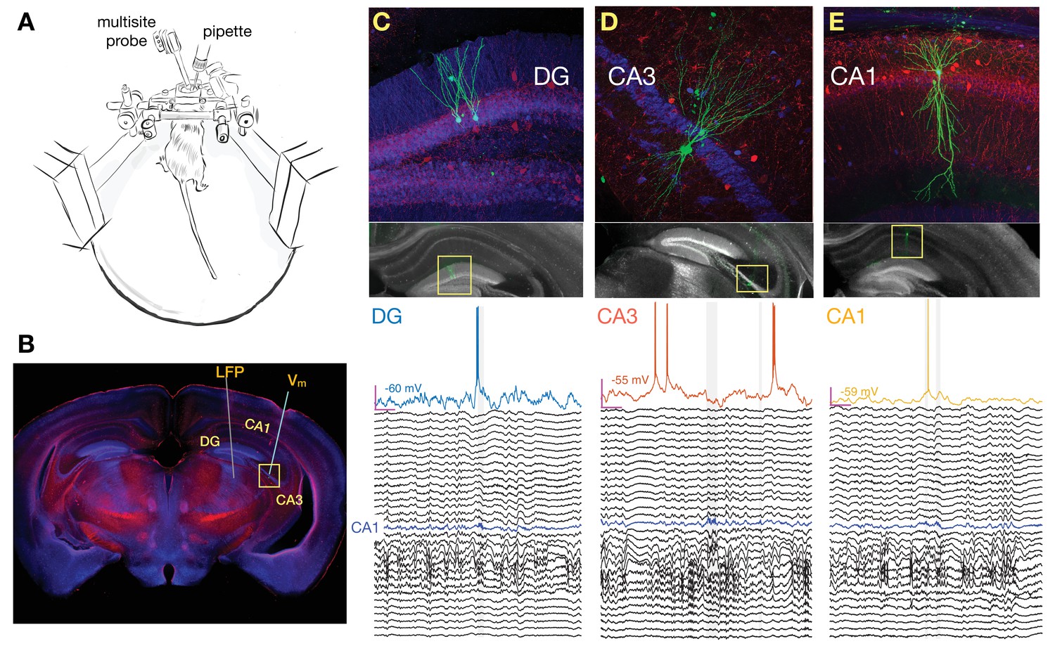
Simultaneous multisite extracellular and whole-cell recordings across hippocampal subfields.
(A) Schematic of setup for simultaneous intracellular and extracellular recordings from awake head-fixed mice free to run on a spherical treadmill. (B) Typical penetration paths of multisite probe for local field potential (LFP) recordings and micropipette (targeting CA3 in this example for the neuron shown in D) for whole-cell recordings. Histological sections were stained for biocytin (green), calbindin (blue), and parvalbumin (red). (C) Examples of histology and recordings. Top: Recorded dentate gyrus (DG) granule cells are labeled with biocytin and their location and morphology is visualized with fluorescence microscopy. Bottom: Membrane potential (Vm) of a DG granule cell together with simultaneous LFP recordings spanning both CA1 and DG. The blue trace marks the pyramidal cell layer of CA1 where ripples are detected and marked by the gray vertical shading. Notice that the cell fires right before the onset of a ripple. The magenta bars indicate 200 ms and 20 mV, and the baseline Vm is reported next to the trace (–60 mV). The vertical spacing between LFP traces is 1 mV. (D) Same as (C), but for a pyramidal neuron in CA3. Notice that the cell is hyperpolarized following the ripple onset. (E) Same as (C), but for a pyramidal neuron in CA1. Notice that the cell fires inside one of two nearby ripples.
-
Figure 1—source data 1
Spiking and membrane properties of recorded neurons.
- https://cdn.elifesciences.org/articles/69596/elife-69596-fig1-data1-v1.xls
Figure 1—figure supplement 1
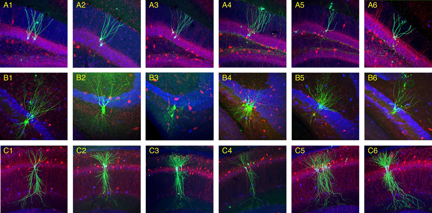
Morphology of recorded neurons.
Histological sections show neurons patched in dentate gyrus (DG; A1–A6), CA3 (B1–B6), and CA1 (C1–C6). Patched cells were filled with biocytin (green), and sections were also stained for calbindin (blue) and parvalbumin (red). Calbindin labels DG axons, seen as a blue band above the pyramidal cell layer in CA3. Notice that in some experiments multiple neurons are patched and labeled. Their identities can still be confirmed when all labeled neurons belong to the same morphological class as illustrated here.
Figure 1—figure supplement 2
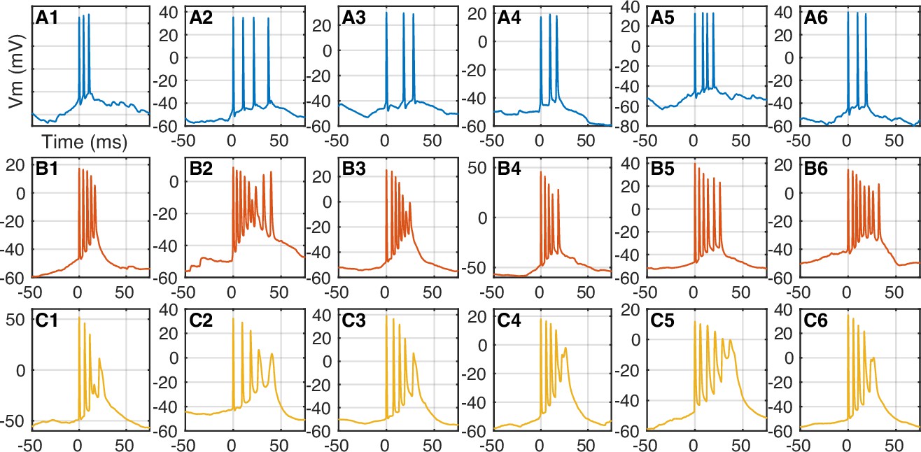
Bursting in recorded neurons.
Examples of spontaneous spike bursts for the labeled neurons in Figure 1—figure supplement 1. Notice that there is little spike amplitude attenuation through the course of the burst in dentate gyrus (DG) granule cells (A1–A6), while CA3 (B1–B6) and CA1 (C1–C6) pyramidal cells produce complex spikes with notable decrease in spike amplitude.
Figure 1—figure supplement 3
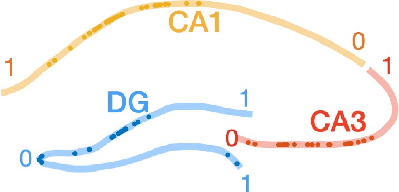
Proximodistal locations of recorded neurons.
Colored lines illustrate the principal cell layers in dentate gyrus (DG), CA3, and CA1 through a coronal section. Each cell is assigned a normalized proximodistal location with 0 corresponding to the proximal end and 1 to the distal end of each subfield (as indicated by the numbers) and then plotted as a dot. This is only a schematic since not all cells were recorded from the same dorsoventral level.
Figure 1—figure supplement 4
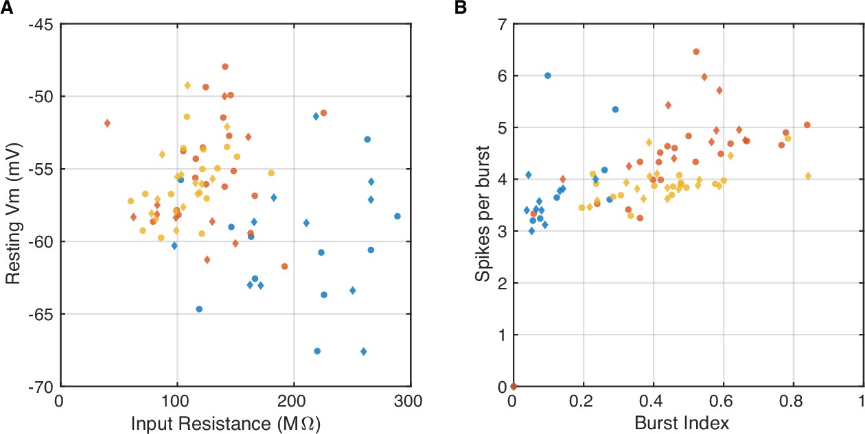
Properties of recorded cells.
(A) Scatter plot shows the input resistance and resting potential for all recorded neurons (markers), color-coded by subfield (dentate gyrus; DG-blue, CA3-red, CA1-yellow). The example neurons from Figure 1—figure supplement 1 are plotted as diamonds, while the remaining cells are plotted as dots. Notice that the morphologically identified cells (diamonds) have similar properties as the rest of the cells from the respective subfield (dots). There were no significant differences between the two groups (p>0.05 t-test; p>0.05 Wilcoxon rank sum test). (B) Same as (A) showing the burst index and average number of spikes per burst for all recorded neurons. The burst index is the fraction of spikes that are part of complex spike bursts. Complex spike bursts are defined as groups of three or more spikes with interspike intervals shorter than 20 ms and decreasing spike amplitudes for at least the first three spikes in the burst. There were no significant differences between the two groups (p>0.05 t-test; p>0.05 Wilcoxon rank sum test).
Figure 2 with 8 supplements
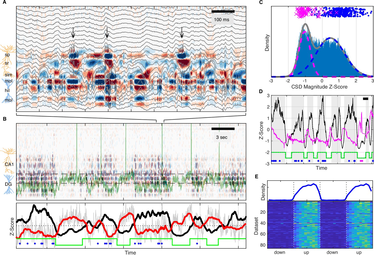
UP and DOWN states modulate slow Vm shifts and ripple occurrence.
(A) Image of current source density (CSD) derived from the local field potential (LFP) traces (gray). Ripples, high-frequency oscillations indicated by the black arrows, are associated with current sinks (red) in stratum radiatum (sr) below the pyramidal cell layer (stratum pyramidale, sp). The bottom third of the image shows large current sources (blue) and sinks (red) within the molecular layers (mol) of dentate gyrus (DG). (B) Top: Image of the CSD on a longer timescale reveals alternating periods of high and low CSD activity. The two interrupted black lines mark the vertical extent of the suprapyramidal molecular layer of DG. The Vm of a CA3 neuron is superimposed in green. Notice that periods of low DG CSD activity (light colors) are associated with Vm depolarization. Bottom: DG CSD activity (black), quantified by averaging the rectified CSD over the molecular layer of DG and smoothing, normalized to a z-score. Subthreshold Vm (gray) for the CA3 neuron and its slow component (red) plotted as z-scores. Notice that the black and red traces are anti-correlated. The green stairstep trace marks epochs of elevated DG CSD activity (UP states) and decreased DG CSD activity (DOWN states). Ripples (blue dots) occur in the UP state. (C) Distribution of DG CSD activity fitted with a two component gaussian mixture. DG CSD activity at ripples (blue dots) and eye blinks (magenta), show preferential association with the UP and DOWN components, respectively. (D) Hidden Markov model (HMM) state detection based on DG CSD activity (black). DG CSD activity is high in the UP state (gray stripes), while the pupil (diameter in magenta) dilates at the onset of the DOWN state and then gradually constricts in the course of the UP state. Ripples and eye blinks are marked by blue and magenta dots, respectively. Horizontal scale bar is 3 s long. (E) (Top) Population average probability density of ripple occurrence as a function of UP and DOWN states (UDS) phase. Notice that ripples occur almost exclusively in the UP state. (Bottom) Rows in the pseudocolor image show the density of ripple occurrence for each dataset (n=86). Densities are replotted over two UDS cycles.
-
Figure 2—source data 1
Probability density of ripple occurrence as a function of UDS phase for each recording.
- https://cdn.elifesciences.org/articles/69596/elife-69596-fig2-data1-v1.xls
Figure 2—figure supplement 1
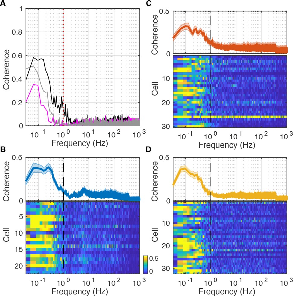
Coherence between rectified dentate gyrus (DG) current source density (CSD) and Vm.
(A) Magnitude-squared coherence of subthreshold Vm and rectified DG CSD (black) or pupil diameter (magenta) for the recording in Figure 2. Coherence of DG CSD and pupil diameter is shown in gray. Magnitude-squared coherence values range between 0 (uncorrelated) and 1 (perfectly correlated) and measure the strength, not the direction, of the correlation at a given frequency. Notice that the signals are coherent below 1 Hz. (B) (Bottom) Each row in the pseudocolor image shows the magnitude-squared coherence of subthreshold Vm and rectified DG CSD for a DG cell. (Top) Population average coherence across all DG cells. (C–D) Same as (B), but for all CA3 (C) and CA1 (D) neurons.
Figure 2—figure supplement 2
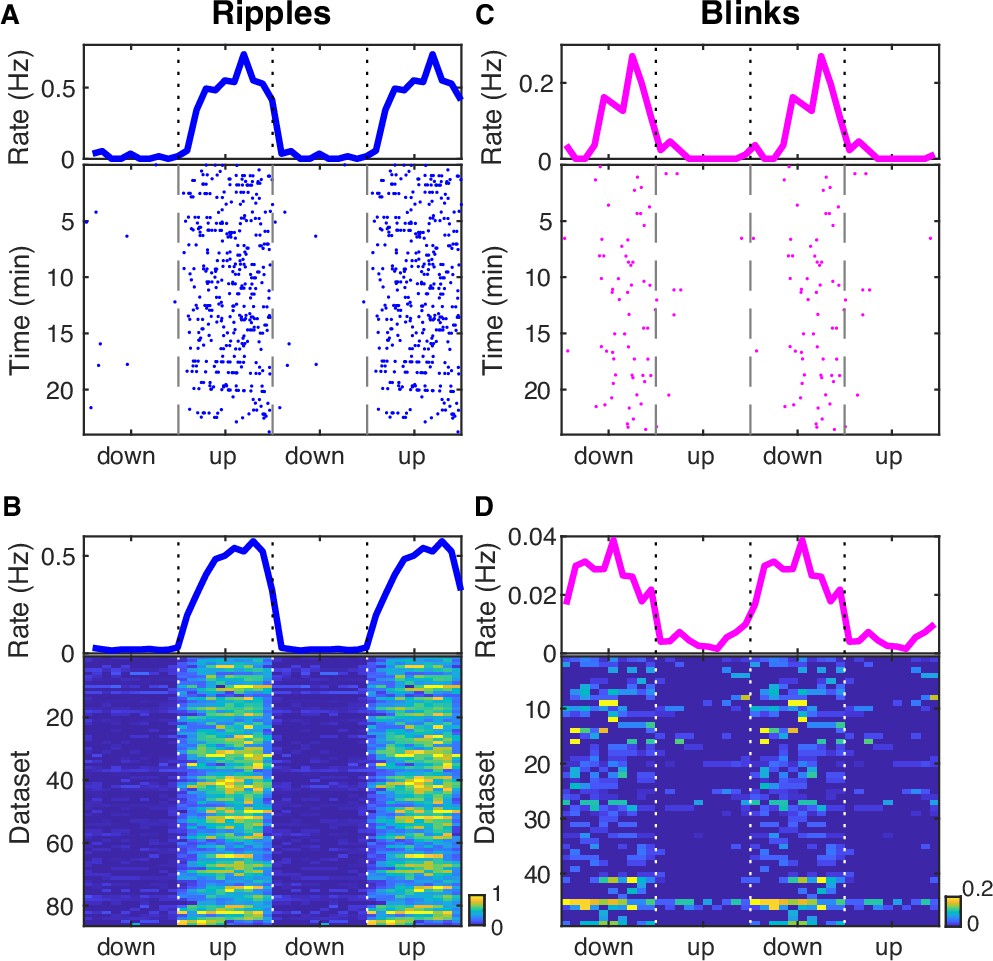
UP and DOWN state (UDS) modulation of ripple and blink occurrence.
(A) (Top) Rate of ripple occurrence as a function of UDS phase for the recording in Figure 2. (Bottom) Dots mark the time and phase of each detected ripple. Notice that almost all ripples occur in the UP state. (B) (Bottom) Rows in the pseudocolor image show the rate of ripple occurrence in each dataset. (Top) Population average rate of ripple occurrence across all datasets. (C) Rate of eyeblinks for the same recording session as (A). Notice that almost all blinks occur in the DOWN state. (D) Rate of eyeblinks across datasets plotted as in (B).
Figure 2—figure supplement 3
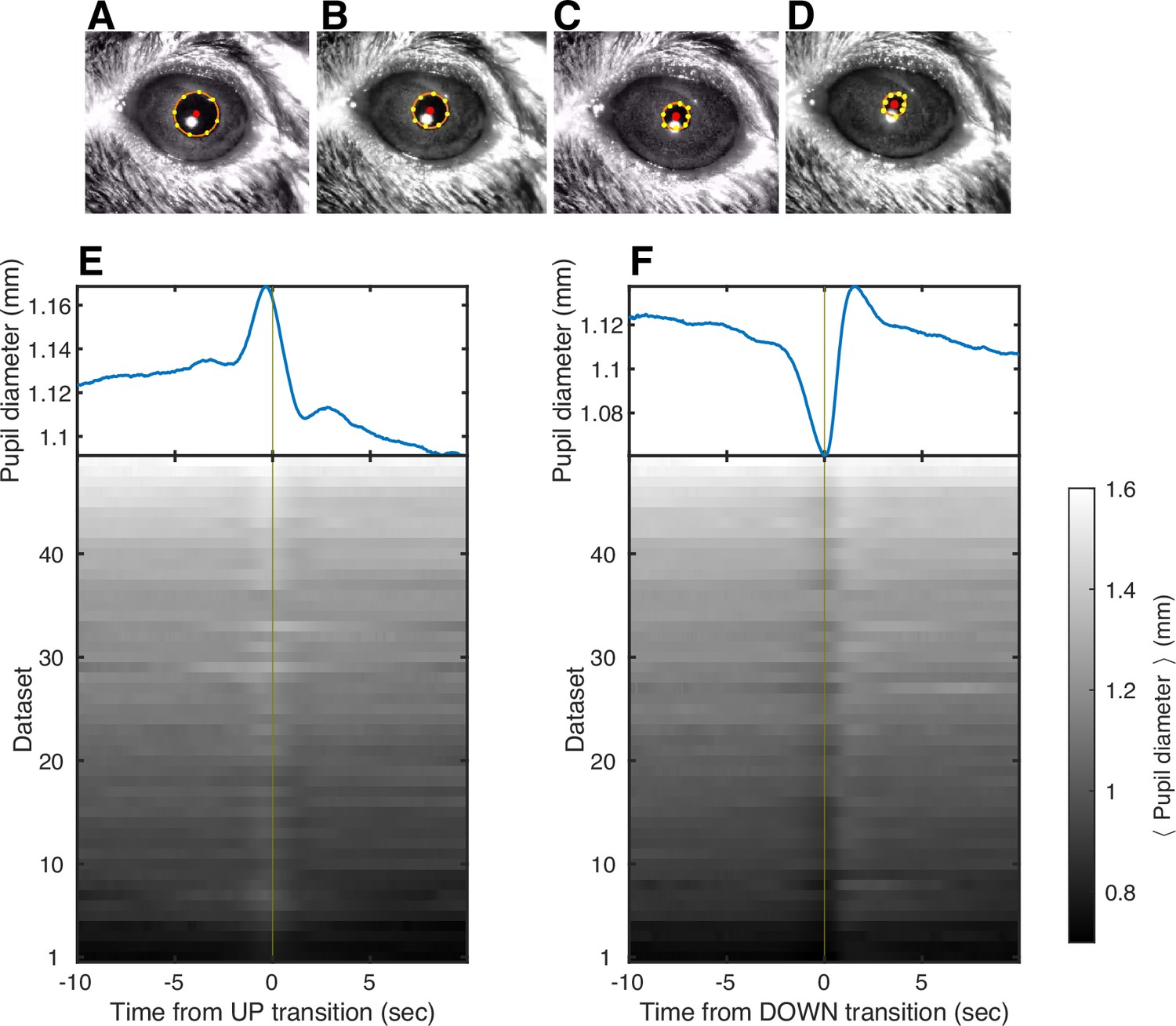
Pupil diameter around UP and DOWN transitions.
(A–D) Examples of pupil tracking. Eight points around the pupil edge were labeled in a subset of frames, and in the remaining frames corresponding points were extracted with DeepLabCut (yellow). The pupil diameter was estimated by fitting a circle (orange) to the extracted points. (E–F) Mean pupil diameter per dataset (bottom) and average across datasets (top) centered on DOWN→UP (E) and UP→DOWN (F) transitions. Notice that the pupil starts dilating at the onset of the DOWN state (F) and is in the process of constricting at the onset of the UP state (E).
Figure 2—figure supplement 4
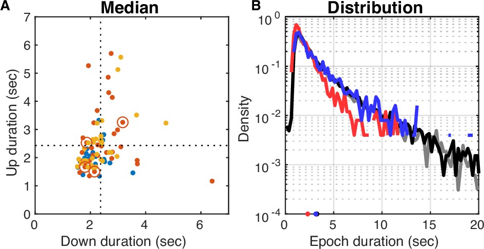
UP and DOWN epoch durations.
(A) Median DOWN epoch duration plotted against median UP epoch duration for each dataset color-coded by subfield of whole-cell target. Population averages are marked by the interrupted lines (UP = 2.43 s, DOWN = 2.37 s). Open circles mark the datasets for which dura resection occurred 3 days before the experiment (no same day anesthesia, UP = 2.24 s, DOWN = 2.25 s). The medians of these four marked datasets were not significantly different from the rest (Wilcoxon rank sum test, p>0.05). (B) Distributions of DOWN (black) and UP (gray) epoch durations pooled across all datasets. Epochs are detected with 250 ms resolution, so the curves at durations shorter than that are affected. Distributions are nearly exponential with similar means (UP = 3.06 s, DOWN = 3.25 s) and standard deviations (UP = 3.57 s, DOWN = 3.48 s). Outliers (15/13053 UP and 2/13139 DOWN epochs with durations longer than 60 s) were excluded. The blue and red lines show the distributions for datasets with no same day anesthesia (means: UP = 2.11 s, DOWN = 3.15 s; standard deviations: UP = 1.95 s, DOWN = 3.11 s).
Figure 2—figure supplement 5
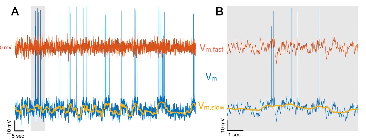
Decomposing membrane potential traces into slow and fast components.
(A) Membrane potential Vm of a CA3 pyramidal cell (blue) decomposed into slow (Vm,slow + Vm,drift in yellow) and fast (Vm,fast in red) components. After spikes are removed from the membrane potential, Vm,slow + Vm,drift is obtained by filtering Vm with a median filter with 1 s window, and Vm,fast = Vm − (Vm,slow + Vm,drift). The 1 Hz cutoff frequency for the decomposition is dictated by the fact that Vm is coherent with brain state indicators up to 1 Hz (Figure 2—figure supplement 1). Vm,drift contains the resting membrane potential and Vm changes on the timescale of minutes, so it only adds a DC offset in the panels above. The short segment indicated by the gray vertical bar is shown in (B).
Figure 2—figure supplement 6
Ripple-triggered average current source density (CSD).
Each panel shows the average CSD triggered on ripple onset (vertical line) corresponding to the datasets from Figure 1—figure supplements 1–2. Horizontal interrupted lines mark the CA1 pyramidal cell layer (top), CA1-dentate gyrus (CA1-DG) border (middle), and DG-thalamus border (bottom). Notice the prominent sink (red) below the CA1 cell layer following the ripple onset. The averaged CSD is less prominent in the DG despite the elevated entorhinal input in the UP state because entorhinal cortex (EC) current transients are not as consistently timed to the ripple onset as the CA1 sharp wave.
Figure 2—figure supplement 7

Rectified current source density (CSD) triggered on UP/DOWN transitions and ripples.
(A1) Rectified CSD in the dentate gyrus (DG) molecular layer (computed by rectifying the raw CSD and averaging over the DG molecular layer; ml sites) is triggered on DOWN→UP transitions for each dataset and displayed as a row in the pseudocolor image. The corresponding average across datasets is shown in the trace above in µA/mm3. Notice the increase in power at the DOWN→UP transition. (A2) Rectified CSD in the DG ml triggered on UP→DOWN transitions. Notice the decrease in power at the UP→DOWN transition. (A3) Rectified CSD in the DG ml triggered on ripples. Notice the shorter time scale and the bump preceding the ripple onset on top of the elevated CSD power.
Figure 2—figure supplement 8

Comparison of large-amplitude irregular activity/small irregular activity (LIA/SIA) and UP/DOWN transitions.
LIA and SIA states and transitions were extracted based on CA1 local field potentials (LFPs) as previously described (Hulse et al., 2017). (A) (Top) Average probability of SIA→LIA transition over the UP and DOWN states (UDS) cycle. (Bottom) Each row shows the probability of SIA→LIA transition for a given dataset. Notice that SIA→LIA transitions are more likely near DOWN→UP transitions. (B) Expected state centered on SIA→LIA transitions. DOWN states are represented by 0 and UP states by 1, so the expected state is equivalent to the UP state probability. Notice that the UP state probability is depressed before and elevated after the SIA→LIA transition. (C) Probability of LIA→SIA transitions over the UDS cycle. Notice that LIA→SIA transitions are very tightly concentrated near the UP→DOWN transition.(D) Expected state centered on LIA→SIA transitions. Notice that the UP state probability is over 90% before the LIA→SIA transition and drops to 0 right after. These observations are consistent with UP states broadly overlapping with LIA and DOWN states with SIA.
Figure 3 with 1 supplement
Entorhinal input to dentate gyrus (DG) is negatively correlated with slow Vm shifts in CA3 in contrast to DG and CA1.
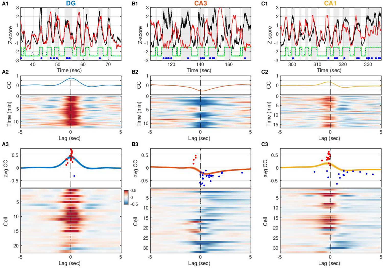
(A1) DG current source density (CSD) activity (black) and slow component (<1 Hz) of subthreshold Vm (red) for an example DG granule cell. Gray vertical stripes and green stairstep trace mark periods classified as UP states. Ripples are marked by the blue dots. Notice that the Vm slow component is modulated in lockstep with the DG CSD. (A2) (Top) Cross-covariance between the slow Vm component of the example cell above and DG CSD activity. (Bottom) Cross-covariances are computed over 30 s sliding windows and displayed as a pseudocolor image. (A3) (Top) Population average cross-covariance of all recorded DG granule cells. Bands around the mean curves show the standard error of the mean (SEM). Dots mark the peak (red) or trough (blue) lag and amplitude of individual cells’ cross-covariance extrema. (Bottom) Cross-covariances for all DG granule cells stacked vertically and displayed as a pseudocolor image. Notice that most traces are peaked near zero lag. In all figures cells are ordered by their ripple-triggered average response (RTA) rank (Figure 6), unless stated otherwise. (B) Same as (A), but for CA3 pyramidal neurons. Notice that the example cell in (B1, B2) and the population overall (B3) have membrane potentials that are anti-correlated with DG CSD activity. (C) Same as (A) and (B), but for CA1 pyramidal neurons. The Vm of many CA1 neurons is positively correlated with DG CSD activity, but the Vm (red) leads the DG CSD (black) as in (C1), so correlation peaks occur at negative lags (C3). A subset of CA1 neurons exhibits negative correlations at positive lags.
-
Figure 3—source data 1
Cross correlation between the slow Vm component and dentate CSD activity for each neuron.
- https://cdn.elifesciences.org/articles/69596/elife-69596-fig3-data1-v1.xls
Figure 3—figure supplement 1
Strength and direction of the correlation between Vm slow component and dentate gyrus (DG) current source density (CSD) activity.
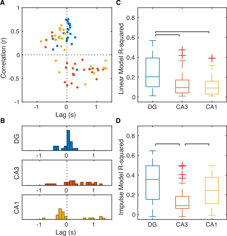
(A) Lag and amplitude at the absolute peak of the cross-covariance between Vm slow and DG CSD activity. Each dot represents a cell and is color-coded by subfield. Notice that for significantly correlated cells (p<0.05 and |r|>0.3: DG 18/22, CA3 18/32, CA1 16/32) most DG (17/18) and CA1 (13/16) cells have a positive peak correlation, while CA3 cells (15/18) have a negative peak correlation. Notice that the peak correlation for many CA1 cells (14/16) occurs at a negative lag (Vm slow leading DG CSD activity). (B) Distribution of peak lags for each subfield. Median lags for cells with significant correlation (p<0.05 and |r|>0.3) for each subfield were: DG (37 ms), CA3 (296 ms), CA1 (–225 ms). (C) Fraction of Vm slow component variance accounted for by its linear correlation to DG CSD activity. The medians are DG (20%), CA3 (9%), CA1 (9%). (D) Fraction of Vm slow component variance that can be explained by an impulse response transfer model with DG CSD activity as input. The medians are DG (36%), CA3 (9%), and CA1 (25%).
Figure 4 with 1 supplement
Entorhinal input differentially modulates slow Vm shifts across hippocampal subfields.
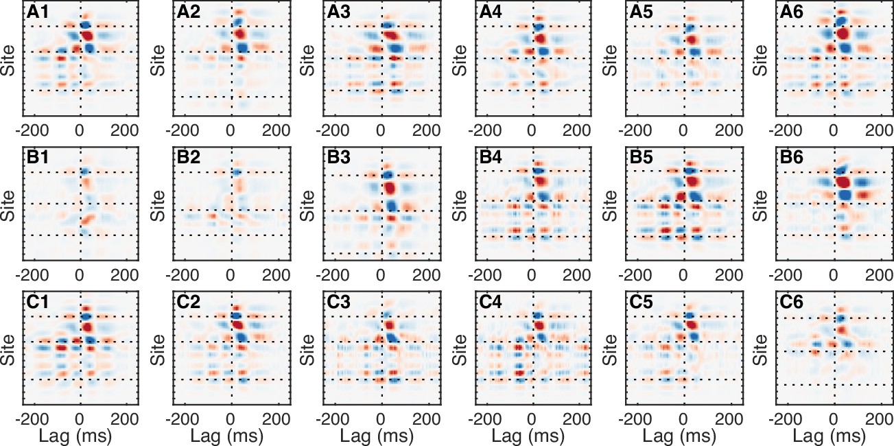
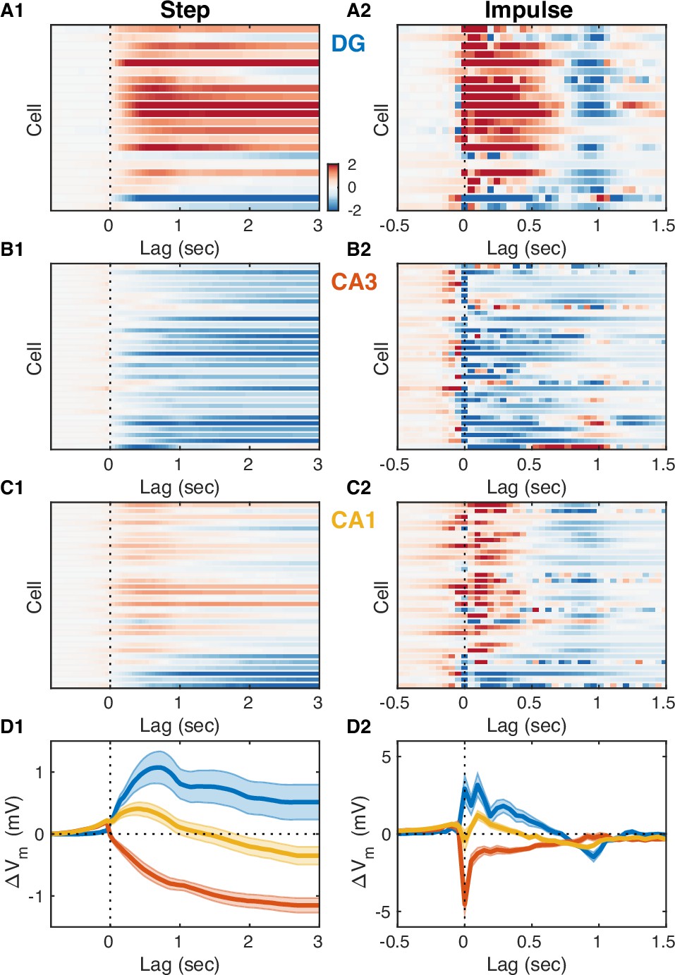
(A1) Each row of the pseudocolor image shows the step response of a linear transfer model describing the effect of dentate gyrus (DG) current source density (CSD) activity on the slow Vm component for a given DG cell. The vertical interrupted line marks the onset of the input step. (A2) Each row shows the impulse responses of the corresponding models in (A1). The vertical interrupted line marks the onset of the impulse. Notice that the majority of DG cells exhibit causal behavior, i.e., the impulse response is near zero for negative lags. (B) Same as (A), but for CA3 pyramidal neurons. Notice that the majority of CA3 neurons hyperpolarize in response to entorhinal cortex (EC) input and some cells exhibit non-causal impulse responses, i.e., some impulse responses have non-zero (positive) values at negative lags. (C) Same as (A) and (B), but for CA1 pyramidal neurons. Notice that some CA1 cells also exhibit non-causal impulse responses. (D) Area-specific population average step response (D1) and impulse response (D2) color-coded by brain area. Bands around the mean curves show the SEM. Notice the distinct responses across hippocampal subfields.
-
Figure 4—source data 1
Vm step and impulse response to dentate CSD activity for each neuron.
- https://cdn.elifesciences.org/articles/69596/elife-69596-fig4-data1-v1.xls
Figure 4—figure supplement 1

Linear prediction of slow Vm component from dentate gyrus (DG) current source density (CSD) activity.
(A1) Data from an example DG granule cell. Vm (with spikes removed) is shown in gray and its slow component in red. DG CSD activity is plotted in black and the UP states are marked by the light gray stripes in the background. All traces are converted to z-scores in order to be compared. (A2) Same as (A1), but the DG CSD trace is omitted and replaced by a linear model prediction of Vm slow (blue) from DG CSD activity. (B) Same as (A), but for an example CA3 pyramidal cell. (C) Same as (A) and (B), but for an example CA1 pyramidal cell.
Figure 5 with 5 supplements
Hippocampal subfields exhibit distinct activity profiles over the UP and DOWN states (UDS) cycle.
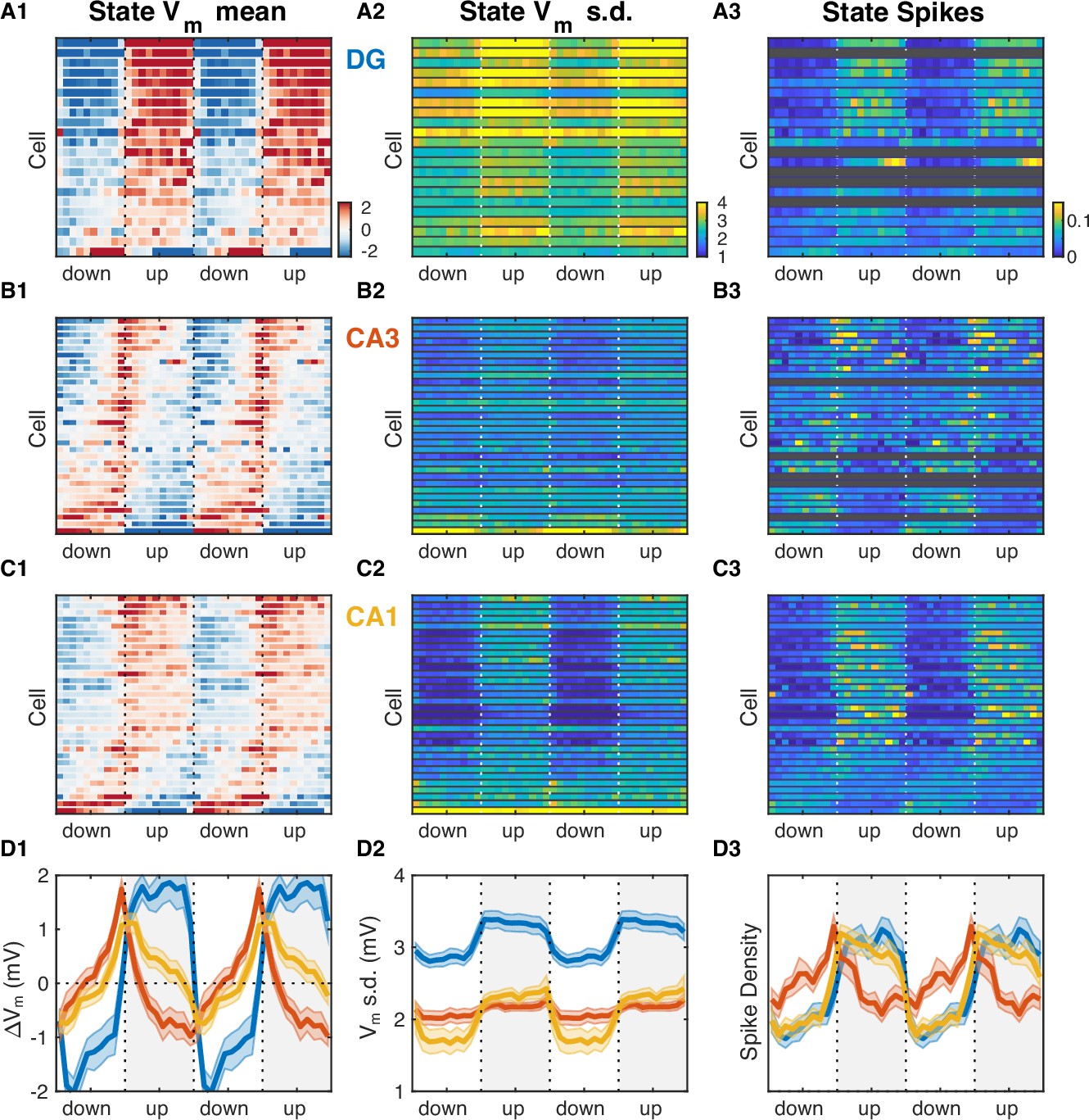
(A1) Vm mean as a function of UDS phase for each dentate gyrus (DG) granule cell displayed as a row in the pseudocolor image. Cells are ordered by the first principal component coefficient of the image matrix (UDS rank). (A2) Fast Vm component standard deviation as a function of UDS phase for DG granule cells. (A3) Observed spiking probability for all DG granule cells displayed as a pseudocolor image. Grayed out rows correspond to cells that fired fewer than 100 spikes. (B) Same as (A), but for CA3 pyramidal neurons. Notice that CA3 neurons are maximally hyperpolarized and have lowest firing probability at the end of the UP phase when the rate of ripple occurrence is highest (Figure 2E). (C) Same as (A) and (B), but for CA1 pyramidal neurons. (D) Area-specific population averages color-coded by brain area. (D1) Population average Vm means. (D2) Population average fast Vm component standard deviations. (D3) Population average spiking probability. Bands around the mean curves show the SEM.
-
Figure 5—source data 1
Vm and spiking responses across UP and DOWN states for each neuron.
- https://cdn.elifesciences.org/articles/69596/elife-69596-fig5-data1-v1.xls
Figure 5—figure supplement 1
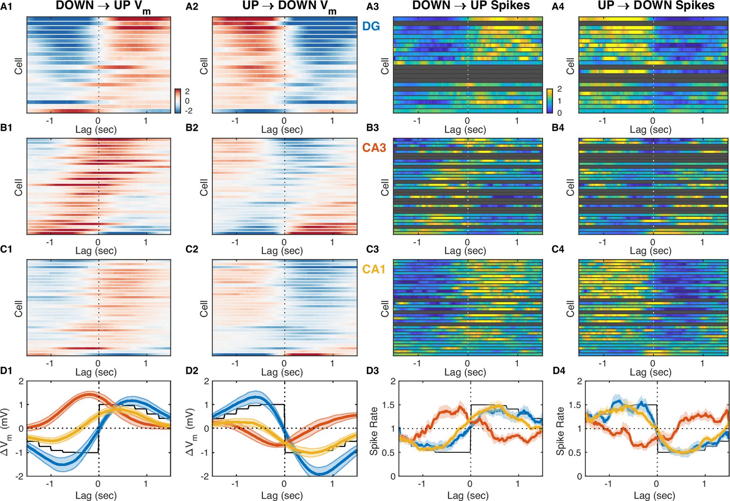
Vm and spiking responses to UP and DOWN states (UDS) transitions reveal ordering in subfield activation.
(A1) Mean slow Vm component (Vm,slow) triggered on DOWN→UP transitions for each DG granule cell displayed as a row in the pseudocolor image. Cells are ordered by UDS rank as in Figure 5. Notice that the Vm of most dentate gyrus (DG) granule cells shifts from hyperpolarized (blue) to depolarized (red) at the UP transition (interrupted vertical line). Color limits in all Vm panels are ± 2.5 mV. (A2) Same as A1, but triggered on UP→DOWN transitions. Notice that in DG the Vm responses to DOWN state transitions are mostly mirror symmetric to the responses to UP transitions. (A3) Spiking responses to DOWN→UP state transitions for all DG granule cells. The perievent time histogram (PETH) for each neuron is normalized to a baseline rate of 1 Hz, so the colors represent the relative modulation of each cell’s baseline firing rate. Notice that firing in the DG is depressed before (blue) and elevated following (yellow) the UP state transition. Grayed out rows correspond to cells with insufficient firing to compute a meaningful PETH. (A4) Same as (A3), but triggered on UP→DOWN transitions. Notice the sharp decrease of firing right at the onset of the DOWN state. (B) Same as (A), but for CA3 pyramidal neurons. Notice that many CA3 cells are already depolarized and have increased firing before the onset of the UP transition. (C) Same as (A) and (B), but for CA1 pyramidal neurons. (D) Area-specific population average Vm responses to UP state transitions (D1), DOWN state transitions (D2), and spiking responses to UP transitions (D3) and DOWN transitions (D4). Bands around the mean curves show the standard error of the mean. Black traces show the average state at each lag with the DOWN and UP states represented by –1 and 1 in (D1 and 2), 0.5 and 1.5 in (D3 and 4).
-
Figure 5—figure supplement 1—source data 1
Vm and spiking responses to UDS transitions for each neuron.
- https://cdn.elifesciences.org/articles/69596/elife-69596-fig5-figsupp1-data1-v1.xls
Figure 5—figure supplement 2
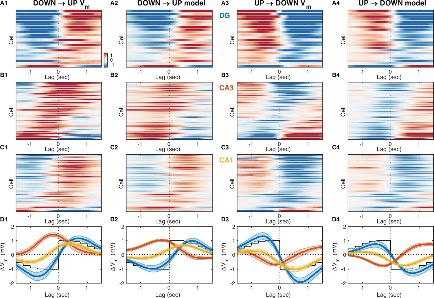
Vm and transfer model responses at UP and DOWN state (UDS) transitions.
(A1–D1) Observed Vm responses at DOWN→UP transitions. Data are replotted from Figure 5—figure supplement 1 for comparison. In all panels cells are ordered by UDS rank is in Figure 5. (A2–D2) Transfer model responses at DOWN→UP transitions simulated from the observed dentate gyrus (DG) current source density (CSD) activity. (A3–D3) Observed Vm responses at UP→DOWN transitions (replotted from Figure 5—figure supplement 1 for comparison). (A4–D4) Transfer model responses at UP→DOWN transitions simulated from the observed DG CSD activity. Bands around the mean curves show the SEM.
-
Figure 5—figure supplement 2—source data 1
Slow Vm and transfer model responses to UDS transitions for each neuron.
- https://cdn.elifesciences.org/articles/69596/elife-69596-fig5-figsupp2-data1-v1.xls
Figure 5—figure supplement 3
UP and DOWN state (UDS) modulation of Vm fluctuations.
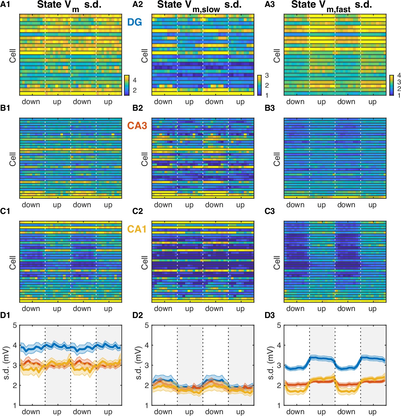
(A1) Vm standard deviation (s.d.) as a function of UDS phase for dentate gyrus (DG) granule cells. Vertical interrupted lines mark state transitions and in all panels data are replotted over two UDS cycles. Cells are ordered according to UDS rank as in Figure 5. (A2) Slow Vm component s.d. as a function of UDS phase for DG granule cells. (A3) Fast Vm component s.d. as a function of UDS phase for DG granule cells. (B) Same as (A), but for CA3 pyramidal neurons. (C) Same as (A) and (B), but for CA1 pyramidal neurons. (D) Area-specific population averages color-coded by brain area. (D1) Population average Vm s.d. (D2) Population average slow Vm component s.d. (D3) Population average fast Vm component s.d.
-
Figure 5—figure supplement 3—source data 1
Vm fluctuations as a function of UDS phase for each neuron.
- https://cdn.elifesciences.org/articles/69596/elife-69596-fig5-figsupp3-data1-v1.xls
Figure 5—figure supplement 4
Resting potential and proximodistal location as predictors of UP and DOWN state (UDS) modulation.
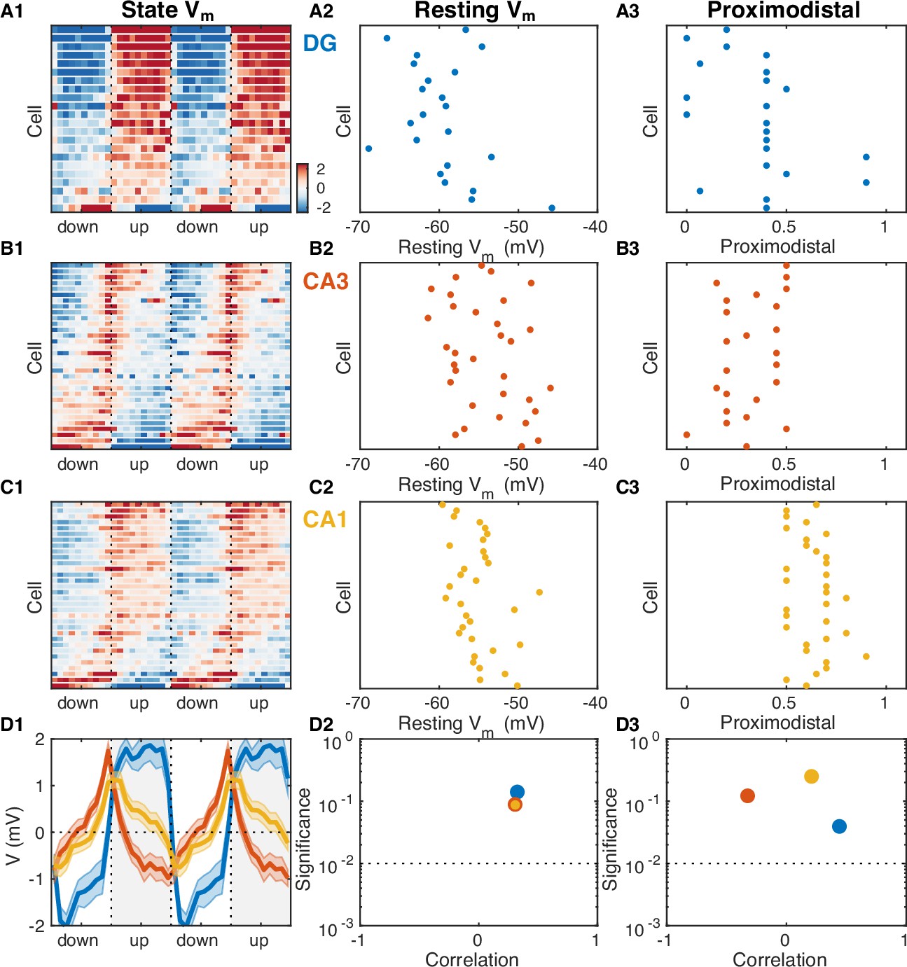
(A1) Vm mean as a function of UDS phase for each dentate gyrus (DG) granule cell displayed as a row in the pseudocolor image. Cells are ordered by their UDS rank (first principal component coefficient of the image matrix). (B1) Scatter plot of DG granule cell resting potential and UDS rank indicate the absence of a strong relation. (C1) Scatter plot of DG granule cell proximodistal location and UDS rank indicate the absence of a strong relation. (B,C) Same as (A), but for CA3 (B) and CA1 (C) pyramidal neurons. (D1) Population average Vm means. (D2) Magnitude and significance of rank order correlation between resting membrane potential and UDS rank for each area. (D3) Magnitude and significance of rank order correlation between proximodistal location and UDS rank for each area. Notice the absence of a significant relation.
Figure 5—figure supplement 5
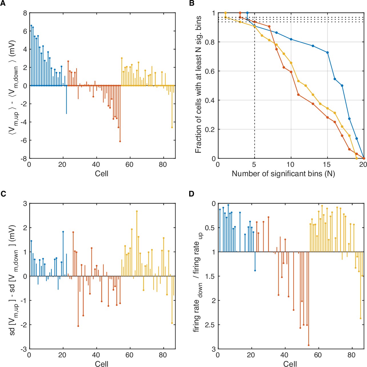
Statistical differences in Vm mean, fast Vm variance, and firing rate across UP and DOWN states (UDS).
(A) Each vertical stem line shows the difference between the mean Vm in the UDS for a given cell. Cells are ordered by UDS rank as in Figure 5 and color coded by subfield (dentate gyrus (DG)-blue, CA3-red, CA1-yellow). Significant differences (p<0.01, t-test) are indicated by dots at the end of the stem lines. The percentage (fraction) of cells with significantly different Vm means were as follows: DG 73% (16/22), CA3 41% (13/32), CA1 44% (14/32). Of those, the proportion of cells with more depolarized Vm in the UP state were: DG 100% (16/16), CA3 31% (4/13), CA1 93% (13/14). The remaining cells were more depolarized in the DOWN state: DG 0% (0/16), CA3 69% (9/13), CA1 7% (1/14). (B) The t-test does not detect Vm modulation by UDS phase that is mirror symmetric with respect to the UDS transitions. To address this we counted the number of UDS phase bins with mean Vm significantly different from the resting Vm for each cell. The lines show the fraction of cells for each subfield with at least N significant bins up to the total number of phase bins (20). We deemed cells with at least 5 significant bins to be UDS modulated, giving the following percentages: DG 95% (21/22), CA3 97% (31/32), CA1 94% (30/32). The UDS modulated cells are marked in panel (A) by dots at the base of the stem lines. (C) Each stem line shows the difference between the standard deviation of the fast Vm component in the UDS for each cell. Significant differences (p<0.01, F-test) are indicated by dots at the end of the stem lines. The proportion of cells with significantly different fast Vm variance were: DG 41% (9/22), CA3 50% (16/32), CA1 53% (17/32). Of those, the proportion of cells with more variable fast Vm in the UP state were: DG 100% (9/9), CA3 44% (7/16), CA1 82% (14/17). The remaining cells had more variable fast Vm in the DOWN state: DG 0% (0/9), CA3 56% (9/16), CA1 18% (3/17). (D) Each stem line shows the ratio of a cell’s firing rate in the DOWN state and UP state. Significant differences (p<0.01, chi-square test) are indicated by dots at the end of the stem lines. The proportion of cells with significantly different firing rates were: DG 91% (20/22), CA3 69% (22/32), CA1 91% (29/32). Of those, the proportion of cells with higher firing rate in the UP state were: DG 75% (15/20), CA3 23% (5/22), CA1 76% (22/29). The remaining cells had higher firing rate in the DOWN state: DG 25% (5/20), CA3 77% (17/22), CA1 24% (7/29).
Figure 6 with 3 supplements
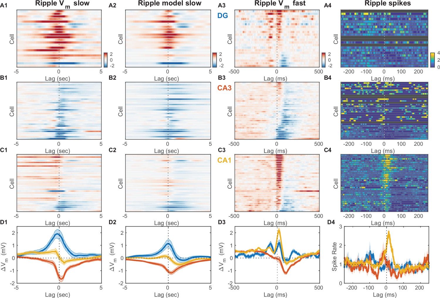
Inhibition marks slow and fast Vm responses near ripples in CA3, unlike dentate gyrus (DG) or CA1.
(A1) Mean slow Vm component triggered on ripple onset for each DG granule cell displayed as a row in the pseudocolor image. Interrupted vertical line marks ripple onset. (A2) Transfer model predicted ripple-triggered slow Vm component as in (A1). (A3) Mean fast Vm components triggered on ripple onset and displayed as in (A1). Notice the two depolarizing peaks at –100 ms and right after ripple onset. Cells in panels (A1−3) are ordered by the first principal component coefficient of the (A3) image matrix (ripple-triggered average [RTA] rank). (A4) Spiking response to ripple onset for DG cells normalized by baseline firing rate. (B) Same as (A), but for CA3 pyramidal neurons. Notice the prominent hyperpolarization for most CA3 neurons present in both the slow and fast Vm component responses. (C) Same as (A) and (B), but for CA1 pyramidal neurons. Notice the prominent depolarization for most CA1 neurons. (D) Area-specific population average slow Vm response (D1), transfer model predicted slow Vm responses (D2), fast Vm response (D3), and spiking response (D4) color-coded by brain area. Bands around the mean curves show the SEM. Notice that modulation by UP and DOWN states (UDS) accounts for the shape of the ripple-triggered Vm response on the timescale of seconds (compare [D1] and [D2]).
-
Figure 6—source data 1
Vm and spiking responses triggered on ripple onset for each neuron.
- https://cdn.elifesciences.org/articles/69596/elife-69596-fig6-data1-v1.xls
Figure 6—figure supplement 1
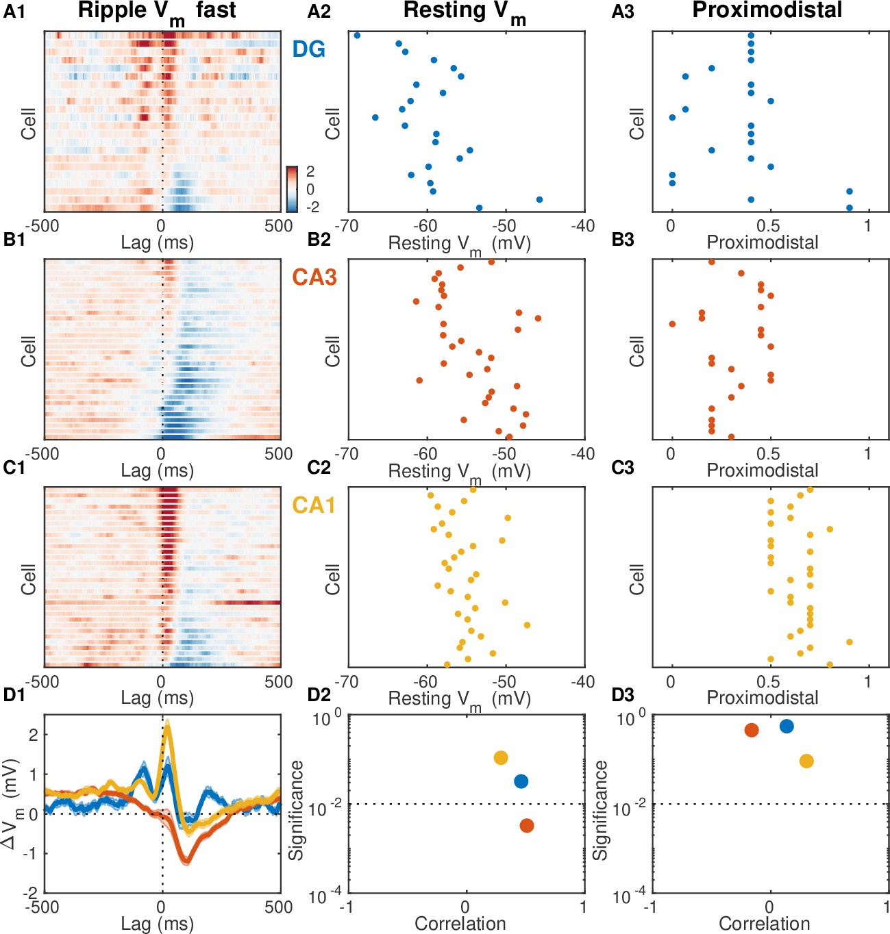
Resting potential and proximodistal location as predictors of ripple modulation.
(A1) Mean fast Vm component triggered on ripple onset for each dentate gyrus (DG) granule cell displayed as a row in the pseudocolor image. Cells are ordered by their ripple-triggered activity (RTA) rank (first principal component coefficient of the image matrix). (A2) Scatter plot of DG granule cell resting potential and ripple rank indicate the absence of a strong relation. (A3) Scatter plot of DG granule cell proximodistal location and ripple rank indicate the absence of a strong relation. (B,C) Same as (A), but for CA3 (B) and CA1 (C) pyramidal neurons. (D1) Population average fast Vm mean responses. (D2) Magnitude and significance of rank order correlation between resting membrane potential and ripple rank for each area. Notice that all areas show a small positive correlation that is only significant in CA3 (red dot). (D3) Magnitude and significance of rank order correlation between proximodistal location and ripple rank for each area. Notice the absence of a significant relation.
Figure 6—figure supplement 2
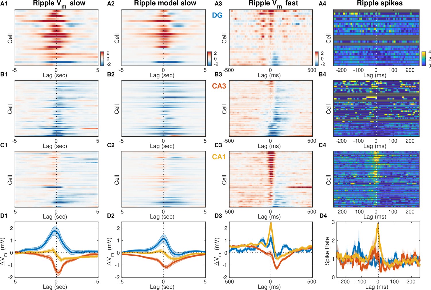
Ripple modulation around ripple peak power.
Same as Figure 6, but lag 0 corresponds to time of peak ripple power, rather than ripple start.
-
Figure 6—figure supplement 2—source data 1
Vm and spiking responses triggered on ripple peak power for each neuron.
- https://cdn.elifesciences.org/articles/69596/elife-69596-fig6-figsupp2-data1-v1.xls
Figure 6—figure supplement 3
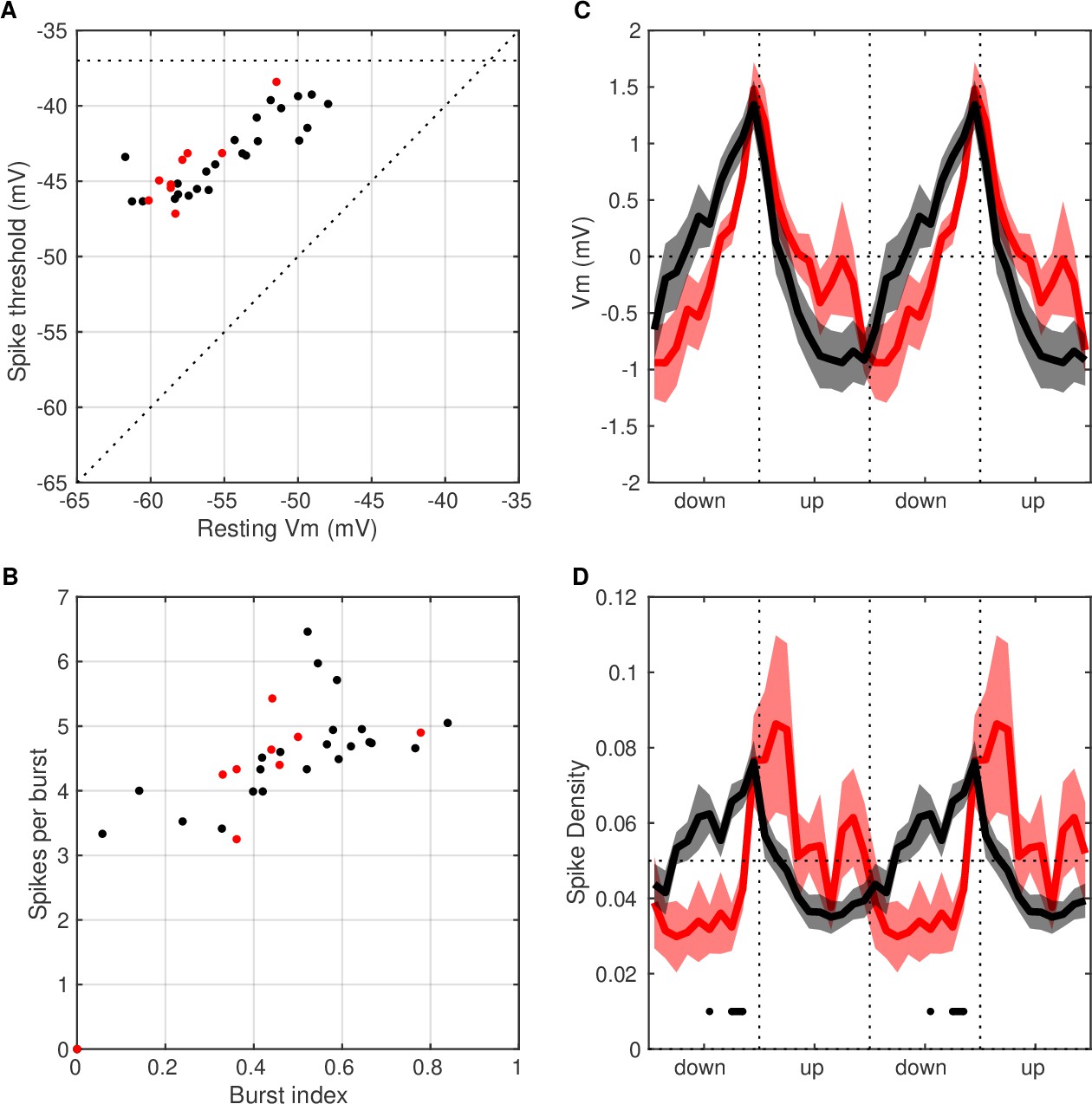
Intrinsic properties and UP and DOWN state (UDS) modulation of CA3 cells that depolarize during ripples.
(A) Resting Vm vs spike threshold of CA3 cells (9/32) showing depolarization in their ripple-triggered average (RTA) response (red) compared to the rest of the CA3 cells (black). These properties were not different between the two groups (t-test, p>0.05). (B) Burst index vs spikes per burst of CA3 cells that depolarized around ripples (red) compared to the rest of the CA3 cells (black). These properties were not different between the two groups (t-test, p>0.05). (C) Average Vm UDS modulation of CA3 neurons that depolarized around ripples (red) compared to the rest of the CA3 cells (black). There were no significant differences between the two groups (t-test, p>0.05). (D) Average spike density UDS modulation of CA3 neurons that depolarized around ripples (red) compared to the rest of the CA3 cells (black). Horizontal black line marks UDS phases with significant differences between the groups (t-test, p<0.01). CA3 neurons that depolarized around ripples had lower firing probability in the DOWN state than the remaining CA3 population.
Figure 7 with 2 supplements
Fast Vm inhibitory responses to ripples scale with CA3 population burst size.
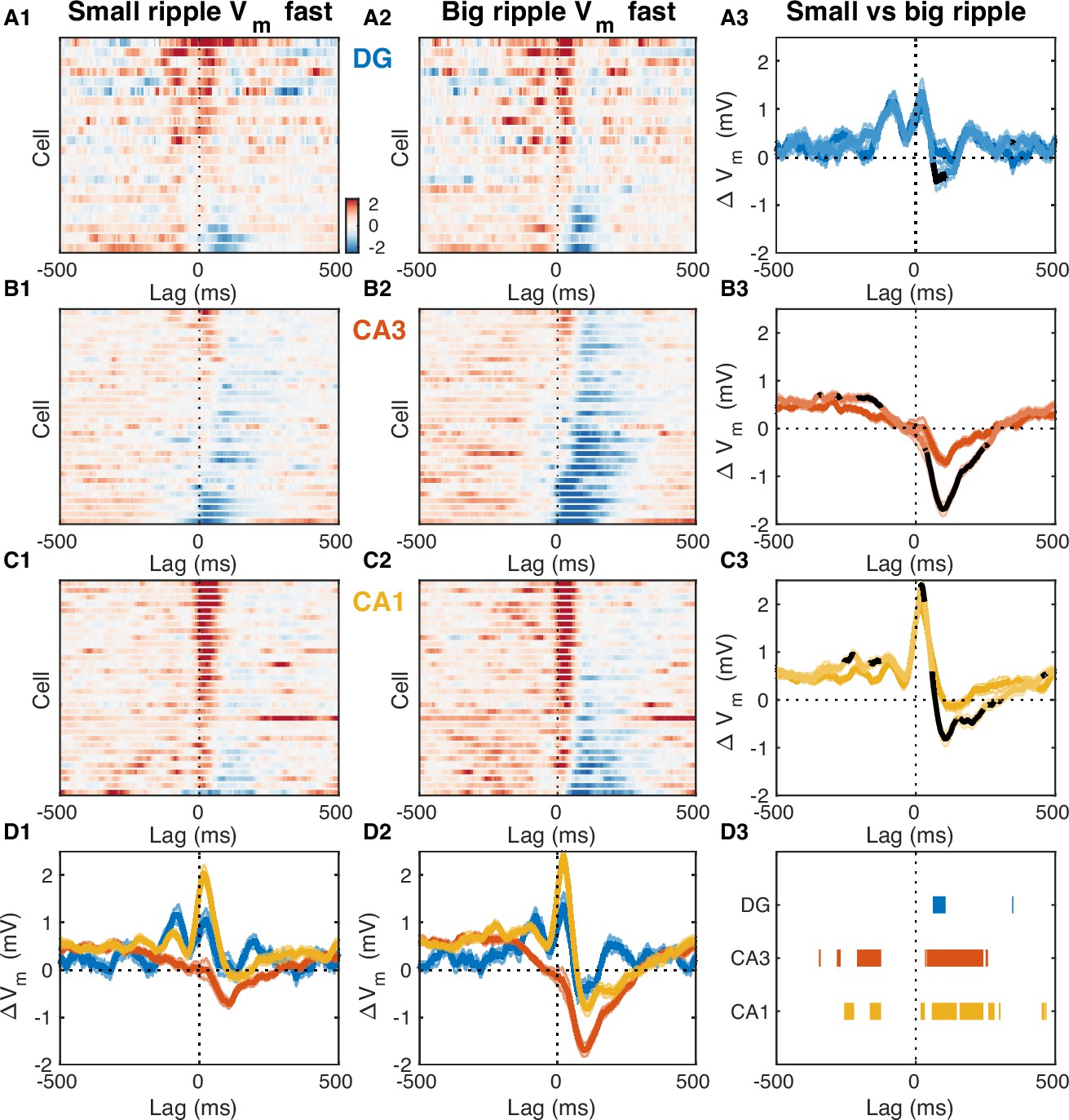
(A1) Mean fast Vm components of dentate gyrus (DG) granule cells triggered on ripples with small (below average) sharp-wave (SPW) amplitudes. (A2) Same as (A1), but for ripples with big (above average) SPW amplitudes. (A3) Comparison of the DG population average response to small and big SPW ripples. Bands around the mean curves show the SEM. Responses to big ripples are shown in darker blue and overlap the responses to small ripples for most time lags. For significant differences the responses to big ripples are highlighted in black (paired t-test, p<0.01). (B) Same as (A), but for CA3 pyramidal neurons. (C) Same as (A) and (B), but for CA1 pyramidal neurons. (D) Area-specific population average responses to small (D1) and big (D2) SPW ripples. Bands around the mean curves show the SEM. (D3) Horizontal bars mark the onset and duration of significant differences between responses to small and big SPW ripples within each area (paired t-test, p<0.01).
-
Figure 7—source data 1
Fast Vm components triggered on onset of ripples with small and large amplitudes.
- https://cdn.elifesciences.org/articles/69596/elife-69596-fig7-data1-v1.xls
Figure 7—figure supplement 1
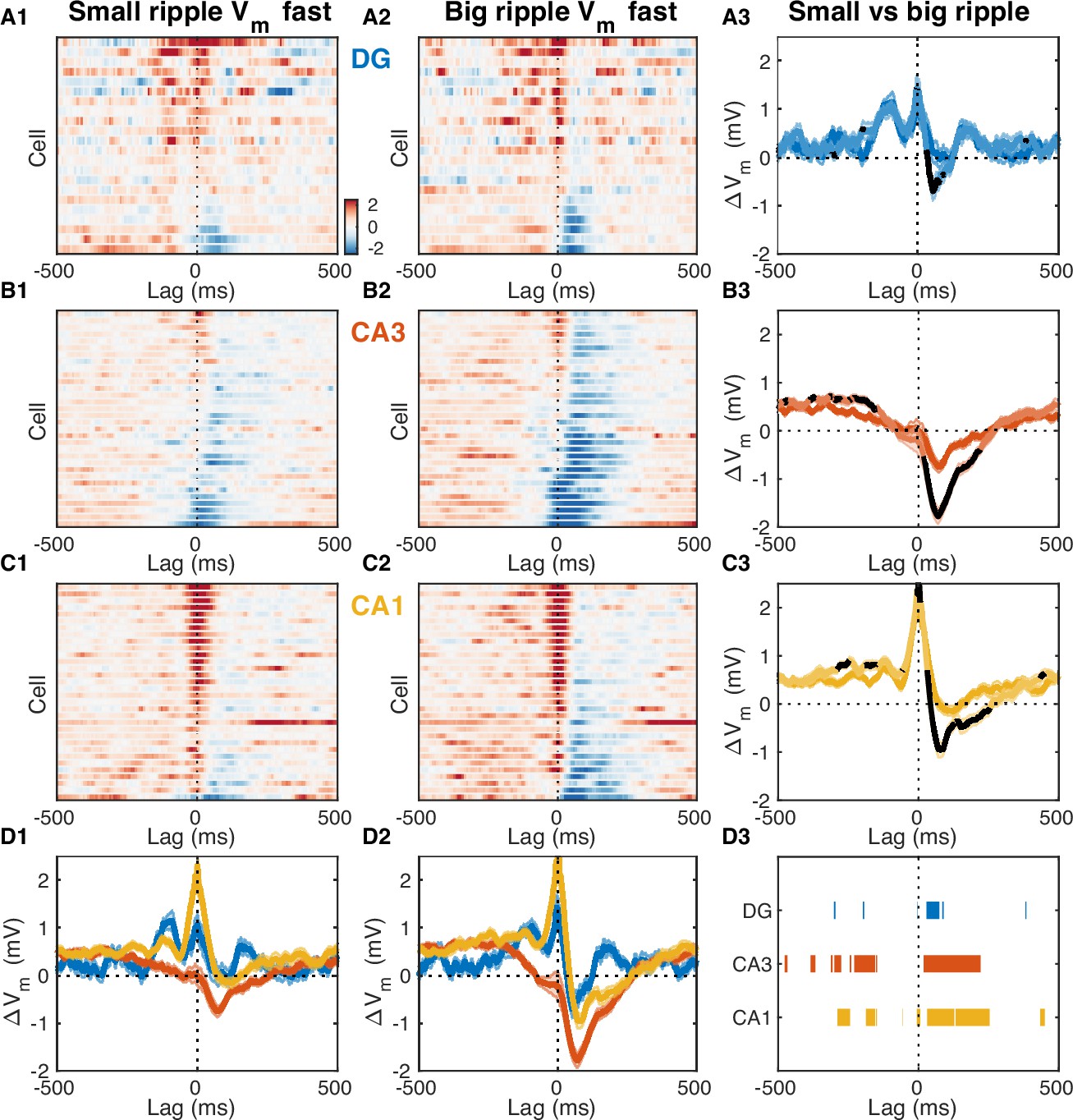
Fast Vm inhibitory responses to ripples scale with CA3 population burst size.
Same as Figure 7, but lag 0 corresponds to time of peak ripple power, rather than ripple onset.
-
Figure 7—figure supplement 1—source data 1
Fast Vm components triggered on peak ripple power of ripples with small and large amplitudes.
- https://cdn.elifesciences.org/articles/69596/elife-69596-fig7-figsupp1-data1-v1.xls
Figure 7—figure supplement 2

Subthreshold ripple modulation around isolated ripples and ripple doublets.
(A1) Mean fast Vm components of dentate gyrus (DG) granule cells triggered on isolated ripples (no ripples occurring within 250 ms from ripple onset). (A2) Mean fast Vm components of DG granule cells triggered on the onset of ripple doublets (second ripple occurring within 250 ms from the start of the first). (A3) Comparison of the DG population averages for isolated ripples (darker hue) vs ripple doublets (lighter hue). Significant differences are highlighted in black. Notice that DG responses are almost identical and the depolarization peak at –100 ms is present before the onset of both isolated ripples and ripple doublets. (B) Same as (A) but for CA3 pyramidal neurons. Notice that while there is significantly more pronounced depolarization preceding ripple doublets, the CA3 response through the course of the first ripple in the doublet matches that seen during isolated ripples. Responses diverge again 200 ms following the onset of the first ripple and an additional hyperpolarization trough is evident at 250 ms due to the second ripple. (C) Same as (A,B) but for CA1 pyramidal neurons. Notice that the secondary depolarization peak in CA1 in response to ripple doublets occurs at 150 ms, halfway between the two hyperpolarization troughs seen in CA3. (D) Area-specific population average responses to isolated ripples (D1) and ripple doublets (D2). (D3) Horizontal bars mark the onset and duration of significant differences between responses to isolated ripples and ripple doublets.
-
Figure 7—figure supplement 2—source data 1
Fast Vm components triggered on the onset of isolated ripples and ripple doublets for each neuron.
- https://cdn.elifesciences.org/articles/69596/elife-69596-fig7-figsupp2-data1-v1.xls
Figure 8
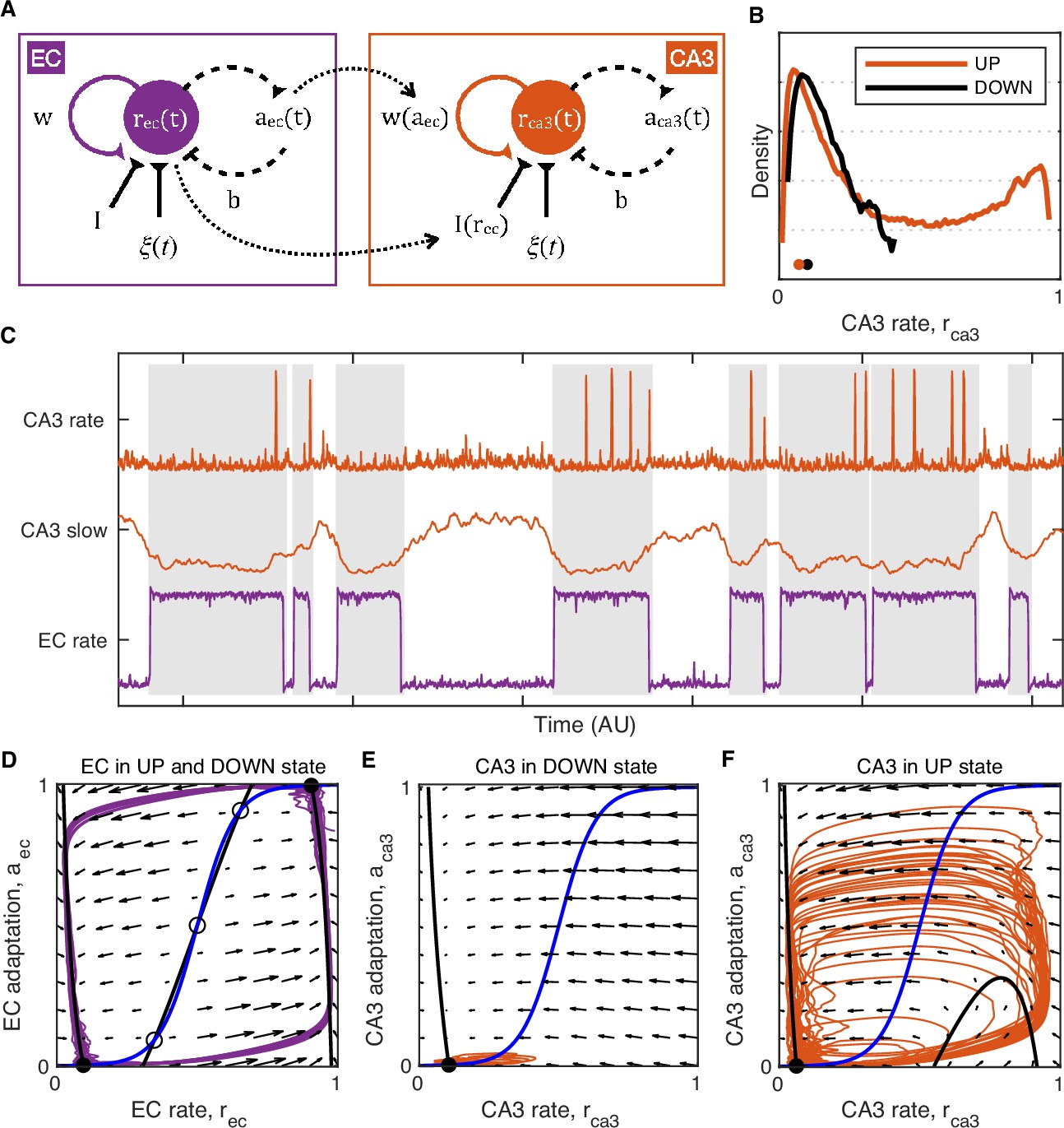
Model of UP and DOWN states (UDS) control of CA3 network excitability.
(A) Idealized model of entorhinal cortex (EC) and CA3 adapting recurrent neural populations. EC activity provides net inhibition to the CA3 population via , possibly due to feedforward inhibition or indirect influence via DG, and modulates the strength of CA3 recurrent excitation via , modeling the effects of UDS-dependent shifts in cholinergic tone on CA3 synaptic transmission. (B) Probability density of the simulated CA3 population rate during EC UP and DOWN states. Notice that the median CA3 population rate is higher in the DOWN than the UP state (black and orange dots) despite the presence of population bursts (rate values near 1) restricted only to the UP state. (C) Example model simulation demonstrating that the EC population exhibits UP and DOWN dynamics while the CA3 population produces transient population bursts (‘ripples’) restricted to the UP state (gray segments). The slow component of the CA3 rate is magnified in the middle to show that mean CA3 activity is higher during the DOWN state and lower during the UP state when population bursts occur. (D–F) Phase plane plots of the model dynamics. The model evolution is governed by the velocity fields displayed as arrows. The model stable (filled circles) and unstable (open circles) fixed points occur at the intersections of the population rate (black) and adaptation (blue) nullclines. Model trajectories are plotted in purple and orange. (D) EC dynamics exhibit two stable fixed points (black circles) corresponding to the UP and DOWN states with noise fluctuations driving transitions between them. (E) CA3 dynamics in the EC DOWN state exhibit a single stable fixed point (black circle) and are not excitable, i.e., noise fluctuations cannot trigger a spike in the population rate. (F) CA3 dynamics in the EC UP state exhibit a single stable fixed point (black circle) at a lower population rate level than in the DOWN state (E), but are excitable, i.e., noise fluctuations can trigger population spikes (‘ripples’).
-
Figure 8—source data 1
Model output time series.
- https://cdn.elifesciences.org/articles/69596/elife-69596-fig8-data1-v1.zip
Author response image 1

Deriving slow envelope signal from AC coupled recordings.
(A) In this example the true CSD signal contains both a slow component (8 Hz) and a fast component (80 Hz) that is amplitude modulated by the slow component. Such phase-amplitude coupling is well known between theta and gamma oscillations in the hippocampus. The true CSD shows a current sink with time-varying magnitude. (B) The power spectral density (PSD) estimate of the signal in (A) shows both the slow (8 Hz) and fast (three peaks near 80 Hz) components. (C) Assume LFP recordings are obtained with a high-pass filter that has eliminated the slow component. Consequently, the estimated CSD signal contains only fast fluctuations. Furthermore, instead of a time-varying current sink it shows quickly alternating sinks and sources (both negative and positive values). The slow component can be visualized as the amplitude envelope (interrupted red line) of the signal. (D) PSD estimate shows that the slow component is absent from the extracted CSD signal. (E) Rectifying the CSD estimate (black) and then filtering (red) approximately recovers the true slow component (red interrupted). This is how the DG CSD activity signal is obtained. (F) PSD estimate of the rectified and filtered CSD signal recovers the slow component (interrupted red vertical line).
Author response image 2
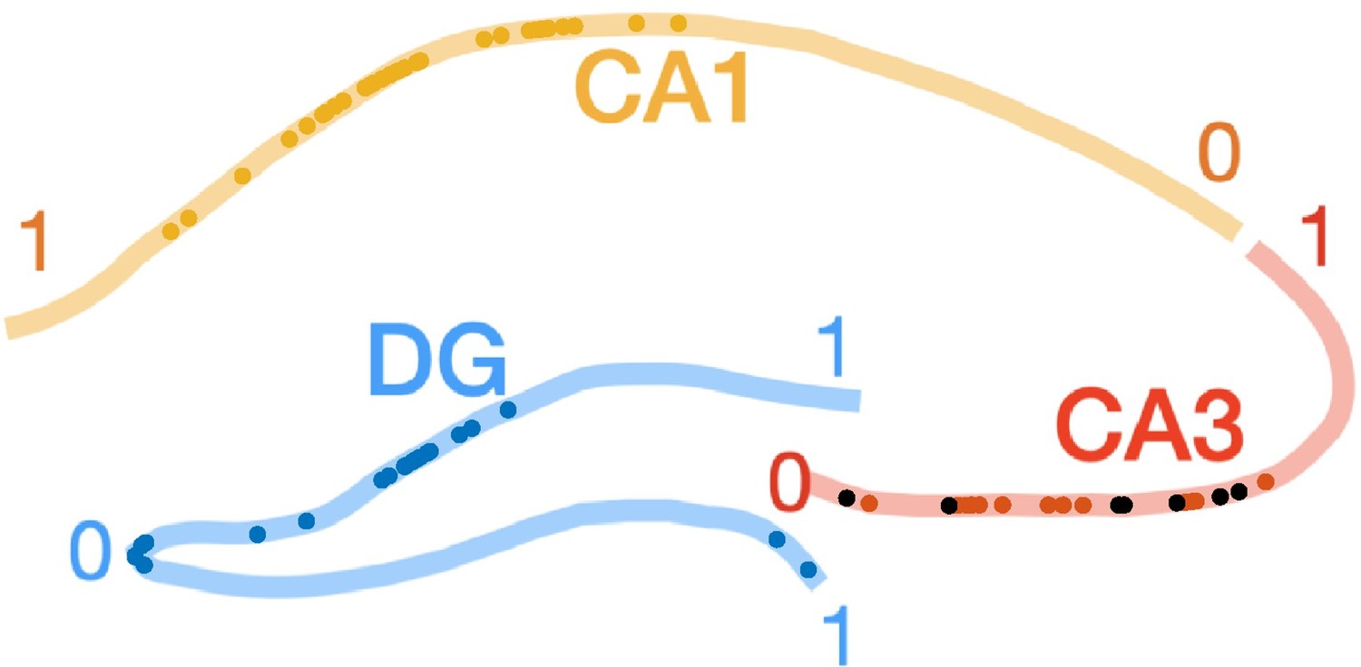
Proximodistal locations of CA3 cells that depolarize during ripples.
Same as Figure 1 - figure supplement 3, but CA3 cells showing depolarization in their ripple-triggered average (RTA) response are marked with black dots. There was no significant difference in the proximodistal locations of these cells compared to the rest of the CA3 population (p > 0.05, t-test).
Additional files
Download links
A two-part list of links to download the article, or parts of the article, in various formats.
Downloads (link to download the article as PDF)
Open citations (links to open the citations from this article in various online reference manager services)
Cite this article (links to download the citations from this article in formats compatible with various reference manager tools)
UP-DOWN states and ripples differentially modulate membrane potential dynamics across DG, CA3, and CA1 in awake mice
eLife 11:e69596.
https://doi.org/10.7554/eLife.69596


