The evolution of strategy in bacterial warfare via the regulation of bacteriocins and antibiotics
- Center for Communicable Disease Dynamics, Harvard TH Chan School of Public Health, Harvard University, United States
- Department of Applied Mathematics and Theoretical Physics, University of Cambridge, United Kingdom
- Department of Veterinary Medicine, University of Cambridge, United Kingdom
- Center for Systems and Control, College of Engineering, Peking University, China
- Institue for Artificial Intelligence, Peking University, China
- School of Mathematics and Statistics, University of Sheffield, United Kingdom
- The Bateson Centre, University of Sheffield, United Kingdom
- Department of Zoology, University of Oxford, United Kingdom
- Department of Biochemistry, University of Oxford, United Kingdom
Figures
Figure 1
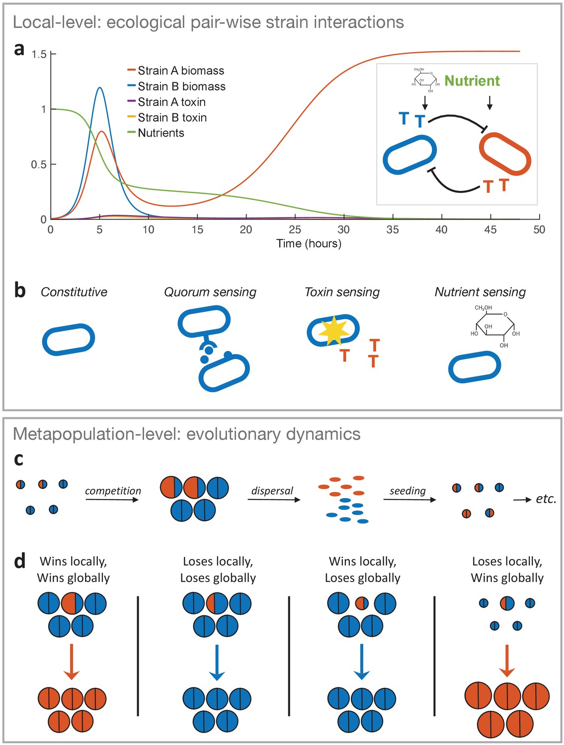
The two-layer modelling framework.
(a) At the ecological timescale, we use differential equations to model the pairwise interactions of strains with competing strains represented here by two single cells in blue and orange. Both strains consume nutrients from a shared pool, and each strain can produce a toxin that inhibits the other strain (represented as coloured ‘T’s). We show an example of the temporal dynamics of a competition between two strains, where strain A wins by investing more into toxin production (fA = 0.3) than strain B (fB = 0.1). All other parameters take the standard values given in Table 1. (b) The differential equation model is used to model four major classes of toxin production strategies. From left to right: Constitutive production without sensing of the environment, sensing clone-mate density (quorum sensing), sensing damage by the competitor’s toxin, and nutrient sensing. Lower panel: At the metapopulation level, we model the long-term evolutionary dynamics of different warfare strategies. (c) Bacterial life cycle assumed for modelling: empty patches are seeded with a small number of cells that then compete, where the outcome is determined according to the local-level model (above). Cells of the two different strategies are shown in blue and orange as circles, where the area represents the number of cells each produces. After competing in the patch for a certain amount of time (24 hours by default), the cells disperse, where the number of cells produced by each strategy determines its frequency in the dispersal phase and new patches. That is, all dispersing cells have the same probability of finding and seeding a new patch, and environmental conditions are identical across patches. Then another competition phase begins and so on (here orange is winning and invading the population). While we show only two different strategies here, we model a metapopulation with more than two strategies when we study the coevolution of attack strategies. (d) Four key outcomes used to predict evolutionary invasion. First case: a rare mutant outcompetes the resident strategy in its patch (orange area is bigger than blue area in the patch). Importantly, the mutant also wins globally, that is, it makes more cells than the average resident in the population, which we take from the number of cells that the resident strategy makes when it meets the same strategy (the size of a semicircle in the all-blue patches). This measure captures resident fitness well because with the mutant being rare and a large number of patches, the resident will nearly always be meeting itself. Second case: mutant loses and, in doing so, makes fewer cells than the average resident. Third case: mutant wins locally, but ends up making very few cells, for example, it redirects a lot of energy into toxins rather than growth. As a result, it does not produce more cells than the average resident strain (i.e. orange area in focal patch is smaller than blue area in all-blue patches). Fourth case: mutant loses locally but produces more cells than the average resident, for example, the mutant is more passive and avoids the strong mutual inhibition of two toxin producers. Thus the mutant wins globally.
Figure 2
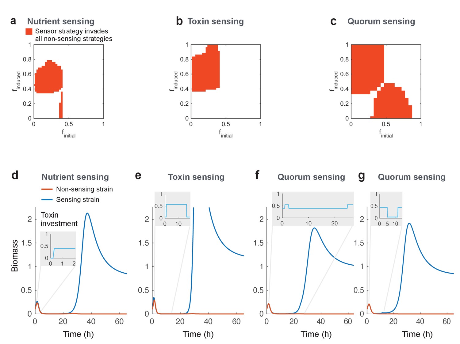
Regulated toxin production outcompetes and evolutionarily replaces constitutive toxin production.
Using a deterministic grid search, we find nutrient-sensing, toxin-sensing, and quorum-sensing strategies that can stably invade the entire range of non-regulated producer strategies (a-c, red areas). In these plots, the effects of two parameters on competitive outcome are shown: finitial, the toxin investment of a sensing strain at the initial state, and finduced, the toxin investment after the signal passes a certain threshold. Red areas indicate combinations of finitial and finduced where at least one threshold value allows stable invasion. Illustrative competitive dynamics are shown for the optimal non-sensing strategy against (d) nutrient-sensing, (e) toxin-sensing, and (f) quorum-sensing (upregulates toxins at high quorum) and (g) quorum-sensing (downregulates toxins at high quorum). Grey insets show investment in toxin production as a function of time. Regulation allows tactics that use toxins more efficiently and effectively than constitutive producers. All parameters take standard values as given in Table 1.
Figure 3
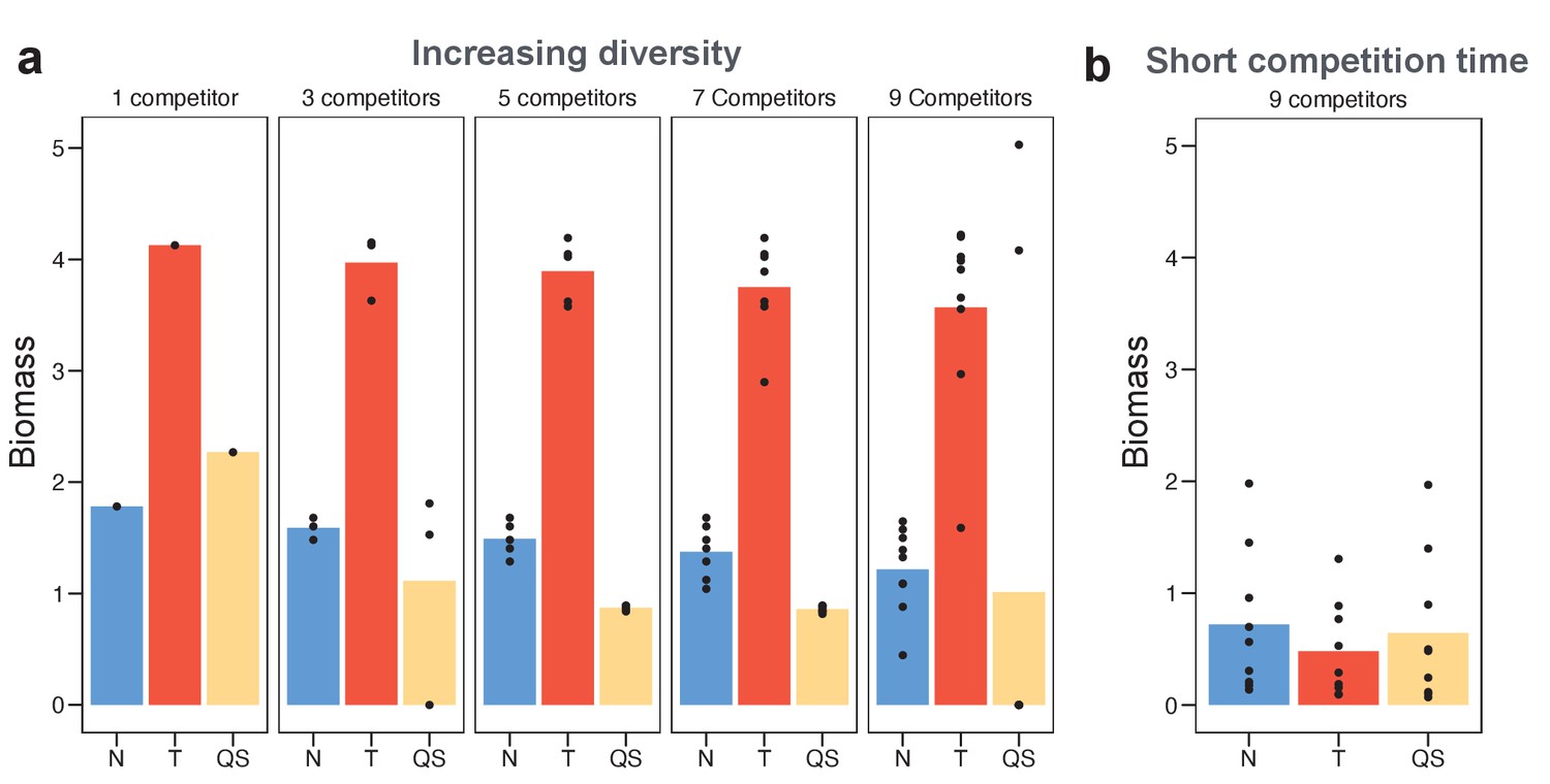
Toxin sensing is the most versatile strategy against a range of different competitor strategies.
(a) We optimised (using a grid search) each of the sensing strategies first against a single constitutive producer (left-hand side panel) and then against an increasing diversity of producers (other panels). As an example, the nine competitors (right-hand side panel) have toxin investment f=0.1,0. 2,…,0.9 and we optimise each of the three sensing strategies in terms of the sum of their final biomasses across all nine competitions. We show the final biomasses of individual competitions as points and the average biomass as bars. The toxin-sensing strain (red coloured bars) performs best, both against the single strategy and against mixtures of strategies. Among the other two sensory strategies, quorum sensing (yellow) has a higher variation of biomass than nutrient sensing (blue) across individual fights. The benefit of sensing toxin is robust for diverse environmental conditions (Appendix 1—figure 7). (b) Shortening the competition time (tend = 6 hr) removes the benefit of toxin sensing. When not mentioned, parameters take the standard values as given in Table 1.
Figure 4
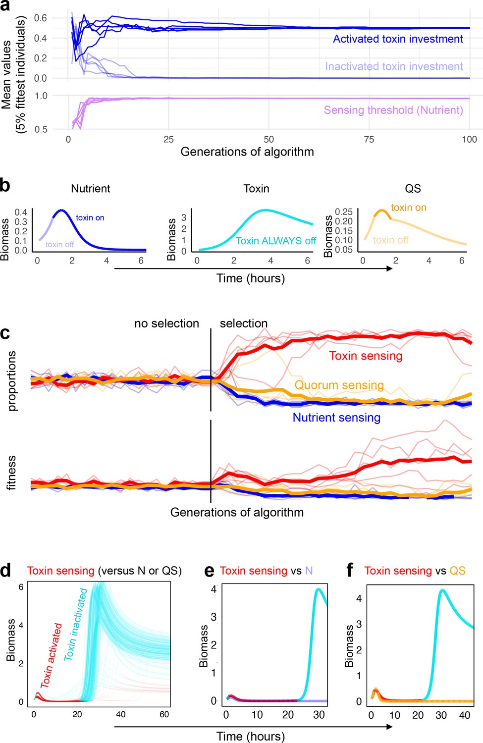
Coevolution of sensing strategies.
Panels a and b follow the evolution of regulation when they compete solely against strains with the same type of regulation, for example, quorum sensing versus quorum sensing; Panels c–f follow evolution when all three types of regulation compete together. (a) Representative example of evolutionary convergence of the sensing parameters for the case of nutrient-sensing strategies competing solely against other nutrient-sensing strains. Displayed is the mean parameter value of the 5% fittest strains at each generation for 10 independent runs of the algorithm. (b) The biomass dynamics of the three evolutionarily stable sensing strategies at equilibrium (when in competition with a strain with an identical strategy). Areas where the dynamics are shown in a pale tone indicate time intervals where toxin was downregulated. For toxin sensing, toxin production remains deactivated thoughout. (c) Evolution in tournaments where all strategies compete against one another, showing the dominance of the toxin sensing strategy. For five independent runs of the tournament the upper panel shows population fraction of the different strategies, the lower panel shows individual fitness averaged per sensing type. The thick lines give the average across runs. The tournament starts with 20 generations (left of the vertical line) without selection, after that, strategies are selected based on their competitive fitness. (d) Winning strategies: shown is the range of dynamics of the optimised toxin sensing strategies against quorum sensing and nutrient-sensing strategies that evolved in one realisation of the tournament. Red and turquoise indicate activated and inactivated toxin production, respectively. (e) Example of a competition between one of the winning toxin-sensing strains meeting a nutrient-sensing strain evolved in the tournament. Red and turquoise, respectively, indicate upregulated and downregulated toxin production for the toxin-sensing strain, other strain is shown in light blue. (f) Example of a competition between one of the winning toxin-sensing strains and a quorum-sensing strain evolved in the tournament. Red and turquoise, respectively, indicate upregulated and downregulated toxin production for the toxin-sensing strain, other strain is shown in yellow. All parameters take standard values as given in Table 1.
Appendix 1—figure 1
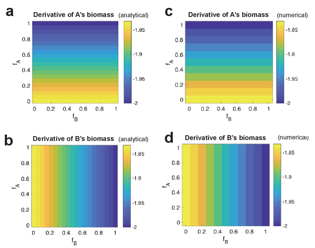
Analytical derivative of strain biomass compared to numerical change in strain biomass.
For different combinations of fA and fB values, analytical derivative of strain A’s biomass (a) and of strain B’s (b). This is shown side-by-side with numerical change in biomass of strain A (c) and strain B (d).
Appendix 1—figure 2
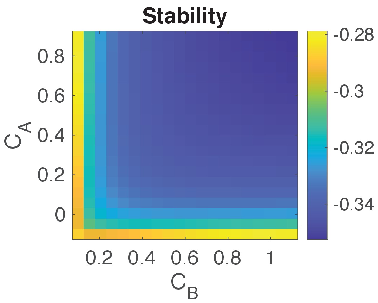
Stability analysis of the system.
Plot shows for a range of values for and the negative of the maximum real part of all the eigenvalues of (−, see details above). Negative values indicate that the system’s state is stable. We choose values for and to be as given in Table 1.
Appendix 1—figure 3
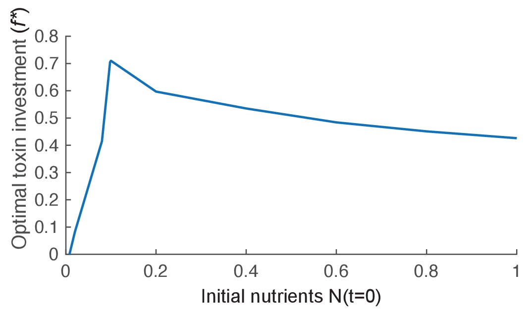
The effect of nutrient availability on optimal toxin investment.
We plot the evolutionary stable investment into toxin over a range of different initial levels of nutrient (N(t=0)). The optimal investment is highest for an intermediate amount of nutrients. Other parameters of the model take the standard values given in Table 1.
Appendix 1—figure 4
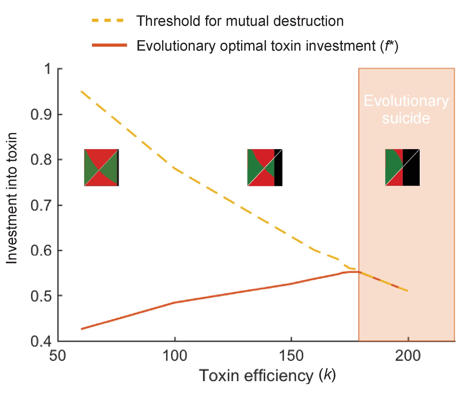
At high toxin efficiency an evolutionary arms race can drive populations towards extinction.
We plot the optimal toxin investment f* (red line) and the investment threshold for mutual destruction fkill (orange line) over different toxin efficiencies (k). Insets show the pairwise invasibility plot for low, medium, and high toxin efficiency. In these plots the x and y axis give the toxin investment (with range 0–1) of the resident and the invading strategy, respectively. Green areas indicate where the invader strategy can successfully replace the resident strategy, red areas indicate where invasion fails. Where the two green and two red triangles have their meeting point at the diagonal line, lies the evolutionarily stable strategy. Black areas indicate where the resident strategy dies off in competition with itself. We see that above a certain toxin efficiency (k = 179), coevolution causes toxin strategies to produce amounts of toxins that are deadly to both competitors. The toxin arms race causes an evolutionary suicide of the population, analogous to mutually assured destruction. All other model parameters take standard value as given in Table 1.
Appendix 1—figure 5

Short competitions favour the evolution of pre-emptive attack.
We investigate the effect of shortening the duration of competitions and ask how this affects the best performing strategies. In nature, the duration of competition will vary depending on the rates of dispersal to new patches. (a) Shortening competition time has little effect on the evolution of constitutive toxin production. (b) Initial investment in regulated toxins increases strongly, favouring pre-emptive attacks. Short competition times select for an increased baseline of aggression in sensing strategies, because it becomes important to overcome a competitor as quickly as possible. (c) At short competition times (6 hr), regulation still remains beneficial and strategies of all three sensing types exist that can invade and evolutionarily replace all constitutive producers (red areas). All parameters take standard values as given in Table 1.
Appendix 1—figure 6
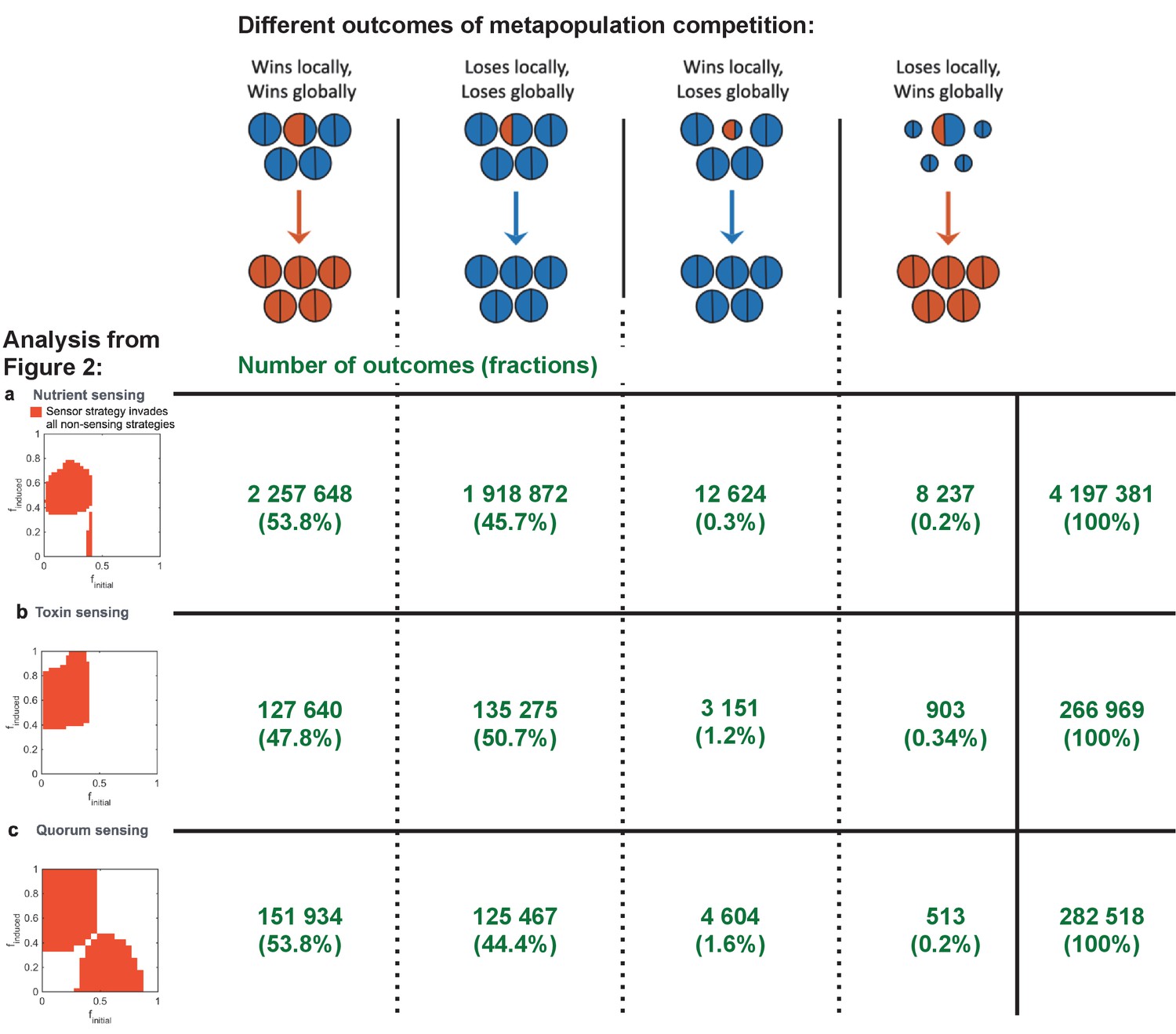
All four competitive dyanmics occur in our simulations.
We enumerate the occurrence of the four different outcomes from the global and local competitions as shown in Figure 1d. Here, the numbers (shown in green) of these outcomes are shown for the simulations used for the three different analyses in Figure 2. We also show in the column to the right the total number of simulations run for each of these analyses, and we give in brackets the proportion of occurrences relative to this total number.
Appendix 1—figure 7
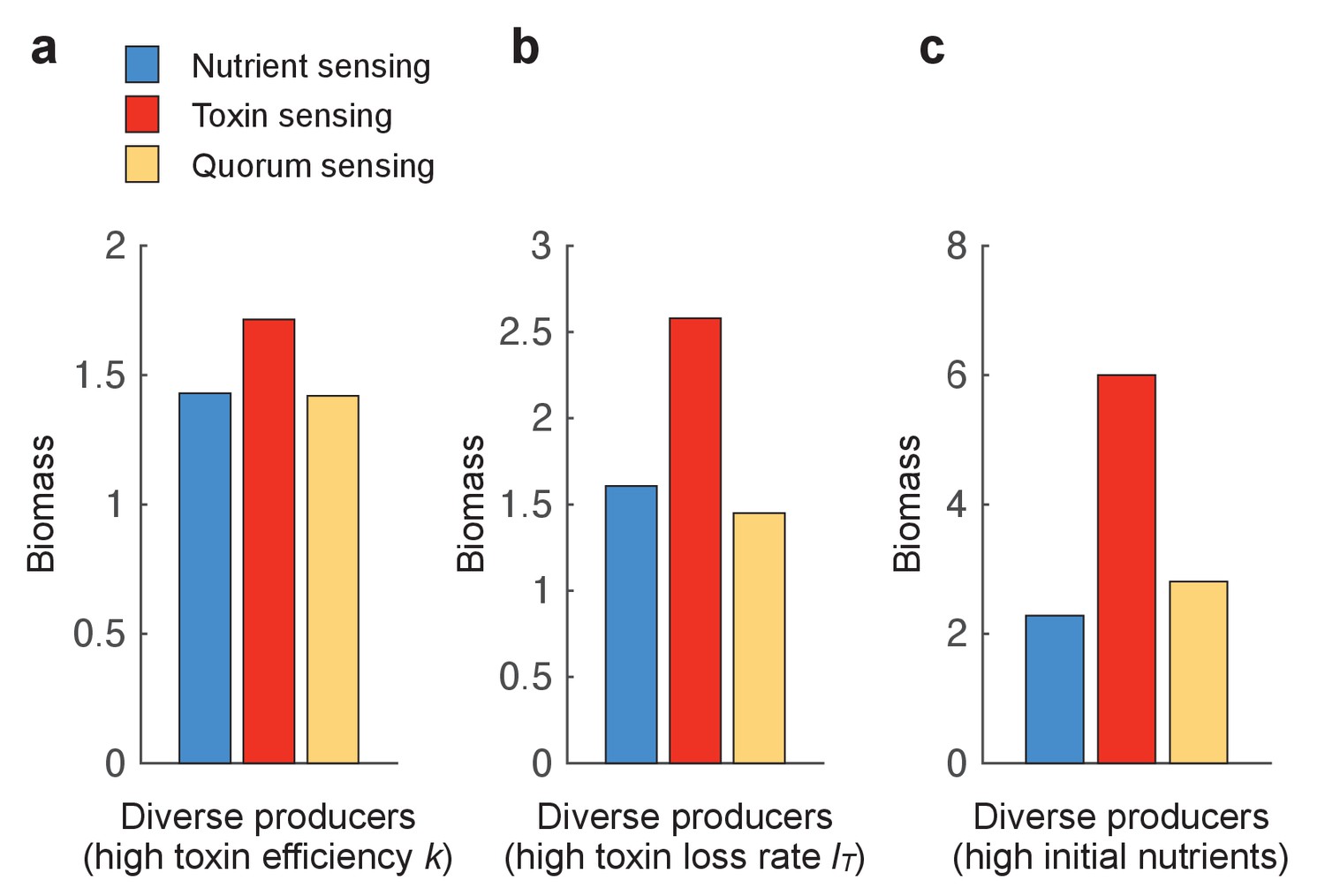
The benefit of toxin sensing is robust across varying environmental conditions.
Figure 3 shows that toxin sensing is the best performing strategy when competing with diverse toxin strategies. Here, we compete the different sensing strategies again against a range of nine constitutive producers (f=0.1, 0.2, …, 0.9) (as in Figure 3b) but under different conditions, which are (a) high killing efficiency of the toxin (k=30), (b) high loss rate of the toxin (l=0.4), and (c) high initial nutrients (N(t=0)=5). All other parameters take standard values as in Table 1.
Appendix 1—figure 8
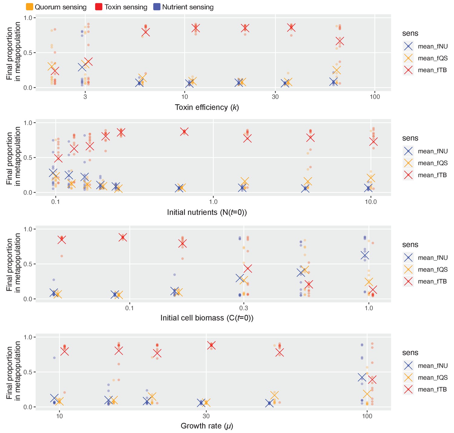
Toxin sensing emerges as the overall winner across wide parameter ranges.
As in Figure 4c, we pit all three sensory strategies against each other in a coevolutionary tournament (genetic algorithm) and we record the proportion of each of the three different types of strategies at the end of the evolution. We show these proportions as coloured dots, and the average proportion across 10 repeat runs of the algorithm as coloured crosses. Finally, we repeat this while varying one model parameter at a time over approximately one order of magnitude, keeping the other parameters as given in Table 1. Toxin-based regulation only fails to show dominance under parameter regimes where selection for the different strategies is relatively weak and noisy in its outcome, that is, low k (toxin has weak effect), high initial cell numbers/low nutrients/slow cell division (few cell divisions per competition cycle and so weaker natural selection).
Appendix 1—figure 9

The evolution of reciprocation (toxin responders) in models of deterministic and stochastic initial strain frequency.
(a) Outcome of the large tournament model with initial strain proportion at 50:50 (as in Figure 4). Shown is the metapopulation proportions of the three different strategy types (toxin sensing in red, quorum sensing in orange, nutrient sensing in blue) over time. (b) and (c) show the same tournament but with competing genotypes arriving stochastically into each competition to create a wide range of initial proportions of each strain ranging from 0 to 1. Density plots on the right show the distribution of initial proportion of strains. The arrival order of the two competing strains is chosen uniformly at random, then the waiting time until the next strain arrives follows an exponential distribution with mean of 20 min (b) and 1 hr (c). We see that, both for the 50:50 mix (a), and under variable initial frequency (b and c) the toxin responders evolve (red line), rather than quorum- (yellow) or nutrient-sensing (blue) strains.
Appendix 1—figure 10
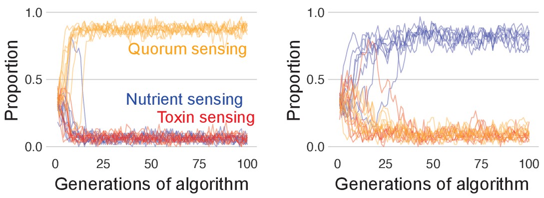
The benefit of toxin sensing over other sensing strategies is lost when competition time is short.
As in Figure 4c, we pit all three sensory strategies against each other in a coevolutionary tournament, but with shortened competition time of 6 hr, which is before the toxin sensor typically recovers (Figure 4d). Lines show the population proportions of the three strategies for 10 runs of the tournament. In the left-hand side, panel quorum sensing is most successful, but which strategy wins changes based upon chance variation in the initial parameter values such that nutrient sensing (right-hand side panel) and toxin sensing (not shown) can also win depending on the parameter ranges set for each sensing type. This indicates that with short competition time, who wins is determined by lucky initial parameter draws that allow one type to dominate the population with a pool of optimised individuals, but the competitive optimum can be reached equally by any of the three sensing types.
Tables
Table 1
Model parameters and their effect on optimal toxin investment.
| Model parameter | Parameter description | Standard value [unit] (notes) | Effect on optimal toxin investment f* |
|---|---|---|---|
| C(t=0) | Initial cell biomass of each strain | 0.1 [gC] | ⬆ |
| N(t=0) | Initial pool of nutrients | 1 [gN] | Intermediate optimum (Appendix 1—figure 3) |
| KN | Saturation constant for nutrient uptake | 5 [gN] | ⬆ |
| µmax | Maximum growth rate | 10 [1/hr] | ⬇ |
| k | Killing efficiency of the toxin | 20 [1/gT*1/hr] | ⬆ |
| lT | Toxin loss rate | 0.1 [1/hr] | ⬇ |
Additional files
Download links
A two-part list of links to download the article, or parts of the article, in various formats.
Downloads (link to download the article as PDF)
Open citations (links to open the citations from this article in various online reference manager services)
Cite this article (links to download the citations from this article in formats compatible with various reference manager tools)
The evolution of strategy in bacterial warfare via the regulation of bacteriocins and antibiotics
eLife 10:e69756.
https://doi.org/10.7554/eLife.69756


