Presynaptic stochasticity improves energy efficiency and helps alleviate the stability-plasticity dilemma
Figures
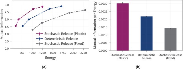
Energy efficiency of model with stochastic and plastic release.
(a) Different trade-offs between mutual information and energy are achievable in all network models. Generally, stochastic synapses with learned release probabilities are more energy-efficient than deterministic synapses or stochastic synapses with fixed release probability. The fixed release probabilities model was chosen to have the same average release probability as the model with learned probabilities. (b) Best achievable ratio of information per energy for the three models from (a). Error bars in (a) and (b) denote the standard error for three repetitions of the experiment.
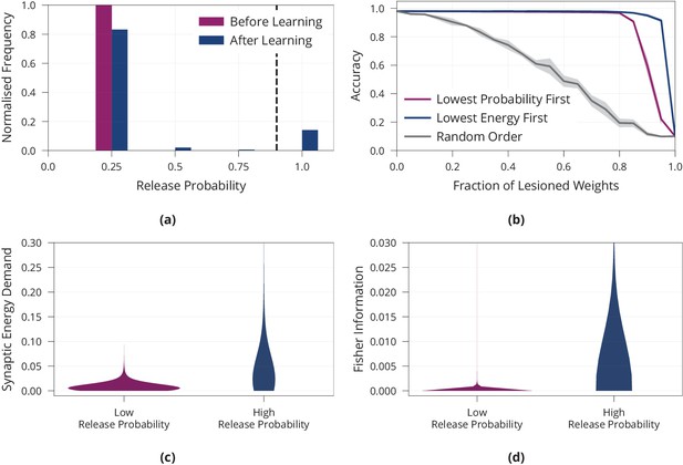
Importance of synapses with high release probability for network function.
(a) Histogram of release probabilities before and after learning, showing that the network relies on a sparse subset of synapses to find an energy-efficient solution. Dashed line at indicates our boundary for defining a release probability as ‘low’ or ‘high’. We confirmed that results are independent of initial value of release probabilities before learning (see Appendix 1—figure 2d). (b) Accuracy after performing the lesion experiment either removing synapses with low release probabilities first or removing weights randomly, suggesting that synapses with high release probability are most important for solving the task. (c) Distribution of synaptic energy demand for high and low release probability synapses. (d) Distribution of the Fisher information for high and low release probability synapses. It confirms the theoretical prediction that high release probability corresponds to high Fisher information. All panels show accumulated data for three repetitions of the experiment. Shaded regions in (b) show standard error.
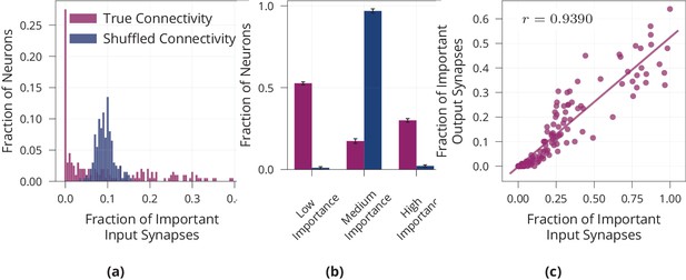
Neuron-level sparsity of network after learning.
(a) Histogram of the fraction of important input synapses per neuron for second layer neurons after learning for true and randomly shuffled connectivity (see Appendix 1—figure 2a for other layers). (b) Same data as (a), showing number of low/medium/high importance neurons, where high/low importance neurons have at least two standard deviations more/less important inputs than the mean of random connectivity. (c) Scatter plot of first layer neurons showing the number of important input and output synapses after learning on MNIST, Pearson correlation is (see Appendix 1—figure 2b for other layers). Data in (a) and (c) are from one representative run, error bars in (b) show standard error over three repetitions.
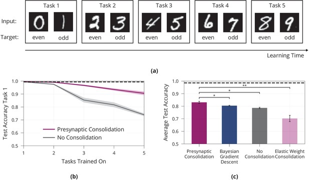
Lifelong learning in a model with presynaptically driven consolidation.
(a) Schematic of the lifelong learning task Split MNIST. In the first task the model network is presented 0 s and 1 s, in the second task it is presented 2 s and 3 s, etc. For each task the model has to classify the inputs as even or odd. At the end of learning, it should be able to correctly classify the parity of all digits, even if a digit has been learned in an early task. (b) Accuracy of the first task when learning new tasks. Consolidation leads to improved memory preservation. (c) Average accuracies of all learned tasks. The presynaptic consolidation model is compared to a model without consolidation and two state-of-the-art machine learning algorithms. Differences to these models are significant in independent t-tests with either (marked with *) or with (marked with **). Dashed line indicates an upper bound for the network’s performance, obtained by training on all tasks simultaneously. Panels (b) and (c) show accumulated data for three repetitions of the experiment. Shaded regions in (b) and error bars in (c) show standard error.
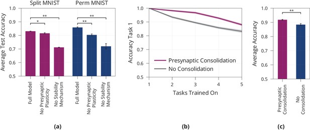
Model ablation and lifelong learning in a standard perceptron.
(a) Ablation of the Presynaptic Consolidation model on two different lifelong learning tasks, see full text for detailed description. Both presynaptic plasticity and synaptic stabilisation significantly improve memory. (b+c) Lifelong Learning in a Standard Perceptron akin to Figure 4b,c, showing the accuracy of the first task when learning consecutive tasks in (b) as well as the average over all five tasks after learning all tasks in (c). Error bars and shaded regions show standard error of three respectively ten repetitions, in (a), respectively (b+c). All pair-wise comparisons are significant, independent t-tests with (denoted by **) or with (denoted by *).
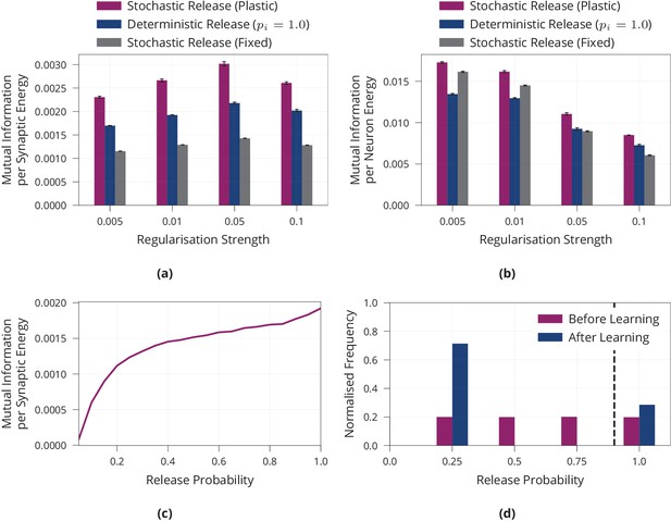
Additional results on energy efficiency of model with stochastic and plastic release.
(a) Mutual information per energy analogous to Figure 1b, but showing results for different regularisation strengths rather than the best result for each model. As described in the main part, energy is measured via its synaptic contribution. (b) Same experiment as in (a) but energy is measured as the metabolic cost incurred by the activity of neurons by calculating their average rate of activity. (c) Maximum mutual information per energy for a multilayer perceptron with fixed release probability and constant regularisation strength of 0.01. This is the same model as ‘Stochastic Release (Fixed)’ in (a), but for a range of different values for the release probability. This is in line with the single synapse analysis in Harris et al., 2012. For each model, we searched over different learning rates and report the best result. (d) Analogous to Figure 2a, but release probabilities were initialised independently, uniformly at random in the interval rather than with a fixed value of 0.25. Error bars in (a) and (b) denote the standard error for three repetitions of the experiment. (c) shows the best performing model for each release probability after a grid search over the learning rate. (d) shows aggregated data over three repetitions of the experiment.
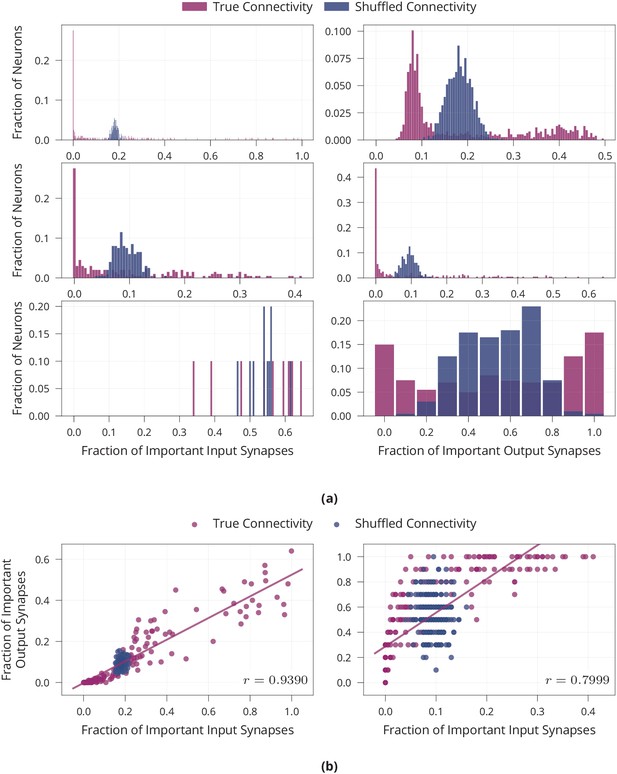
Additional results on neuron-level sparsity of network after learning.
(a) Number of important synapses per neuron for all layers after learning on MNIST. The -th row shows data from the -th weight matrix of the network and we compare true connectivity to random connectivity. Two-sample Kolmogorov-Smirnov tests comparing the distribution of important synapses in the shuffled and unaltered condition are significant for all layers () except for the output neurons in the last layer (lower-left panel) (). This is to be expected as all 10 output neurons in the last layer should be equally active and thus receive similar numbers of active inputs. (b) Scatter plot showing the number of important input and output synapses per neuron for both hidden layers after learning on MNIST. First hidden layer (left) has a Pearson correlation coefficient of . Second hidden layer (right) has a Pearson correlation coefficient of . Data is from one run of the experiment.
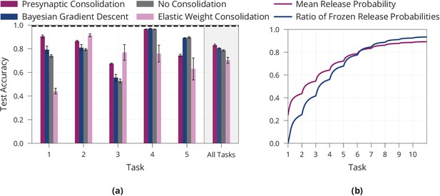
Additional results on lifelong learning in a model with presynaptically driven consolidation.
(a) Detailed lifelong-learning results of various methods on Split MNIST, same underlying experiment as in Figure 4c. We report the test accuracy on each task of the final model (after learning all tasks). Error bars denote the standard error for three repetitions of the experiment. (b) Mean release probability and percentage of frozen weights over the course of learning ten permuted MNIST tasks. Error bars in (a) and shaded regions in (b) show standard error over three repetitions of the experiment.
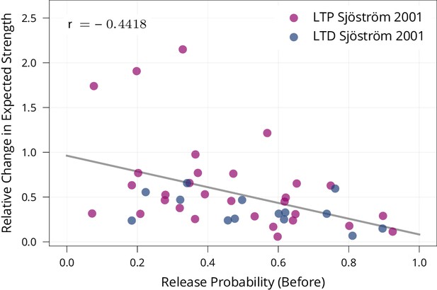
Biological evidence for stability of synapses with high release probability.
To test whether synapses with high release probability are more stable than synapses with low release probability as prescribed by our model, we re-analysed data of Sjöström et al., 2001 from a set of spike-timing-dependent plasticity protocols. The protocols induce both LTP and LTD depending on their precise timing. The figure shows that synapses with higher release probabilities undergo smaller relative changes in expected strength (Pearson Corr. , ). This suggests that synapses with high release probability are more stable than synapses with low release probability, matching our learning rule.
Tables
Lifelong learning comparison on additional datasets.
Average test accuracies (higher is better, average over all sequentially presented tasks) and standard errors for three repetitions of each experiment on four different lifelong learning tasks for the Presynaptic Consolidation mechanism, Bayesian Gradient Descent (BGD) (Zeno et al., 2018) and EWC (Kirkpatrick et al., 2017). For the control ‘Joint Training’, the network is trained on all tasks simultaneously serving as an upper bound of practically achievable performance.
| Split MNIST | Split fashion | Perm. MNIST | Perm. fashion | |
|---|---|---|---|---|
| Presynaptic Consolidation | ||||
| No Consolidation | ||||
| Bayesian Gradient Descent | ||||
| Elastic Weight Consolidation | ||||
| Joint Training |
Additional files
-
Source code 1
Code for presynaptic stochasticity model and baselines.
- https://cdn.elifesciences.org/articles/69884/elife-69884-code1-v2.zip
-
Source data 1
Raw data and code to create figures.
- https://cdn.elifesciences.org/articles/69884/elife-69884-data1-v2.zip
-
Transparent reporting form
- https://cdn.elifesciences.org/articles/69884/elife-69884-transrepform-v2.pdf


