Increased signal-to-noise ratios within experimental field trials by regressing spatially distributed soil properties as principal components
- Donald Danforth Plant Science Center, United States
- School of Biological Sciences, Washington State University, United States
- Department of Biochemistry and Molecular Biology, Colorado State University, United States
- Department of Agronomy and Horticulture, University of Nebraska-Lincoln, United States
- Department of Statistics, Iowa State University, United States
Figures
Figure 1 with 2 supplements
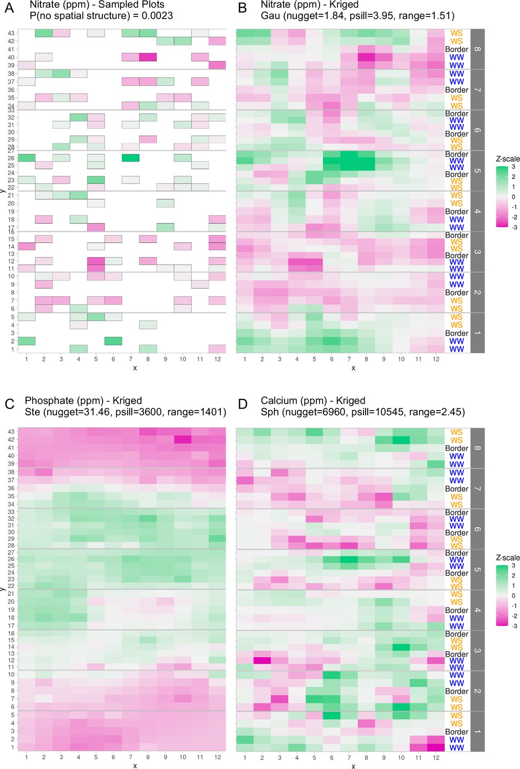
Graphical depictions of field layout where each cell is a plot in the field.
Water treatment is specified on right; WS = water stressed, WW = well-watered. Eight split-plot replicate blocks are denoted in gray vertical bars. Color scale represents data with genotype and treatment removed. Green indicates larger than average, white indicates approximately average, and magenta indicates below average values. (A) Nitrate values are shown for each cell (outlined in gray) that were sampled for soil property analysis. (B) Kriged nitrate values to estimate nitrate levels in unsampled plots. (C, D) Kriged values for phosphate and calcium. Variogram fit of spatial model is indicated with model type, nugget, partial sill, and range.
Figure 1—figure supplement 1
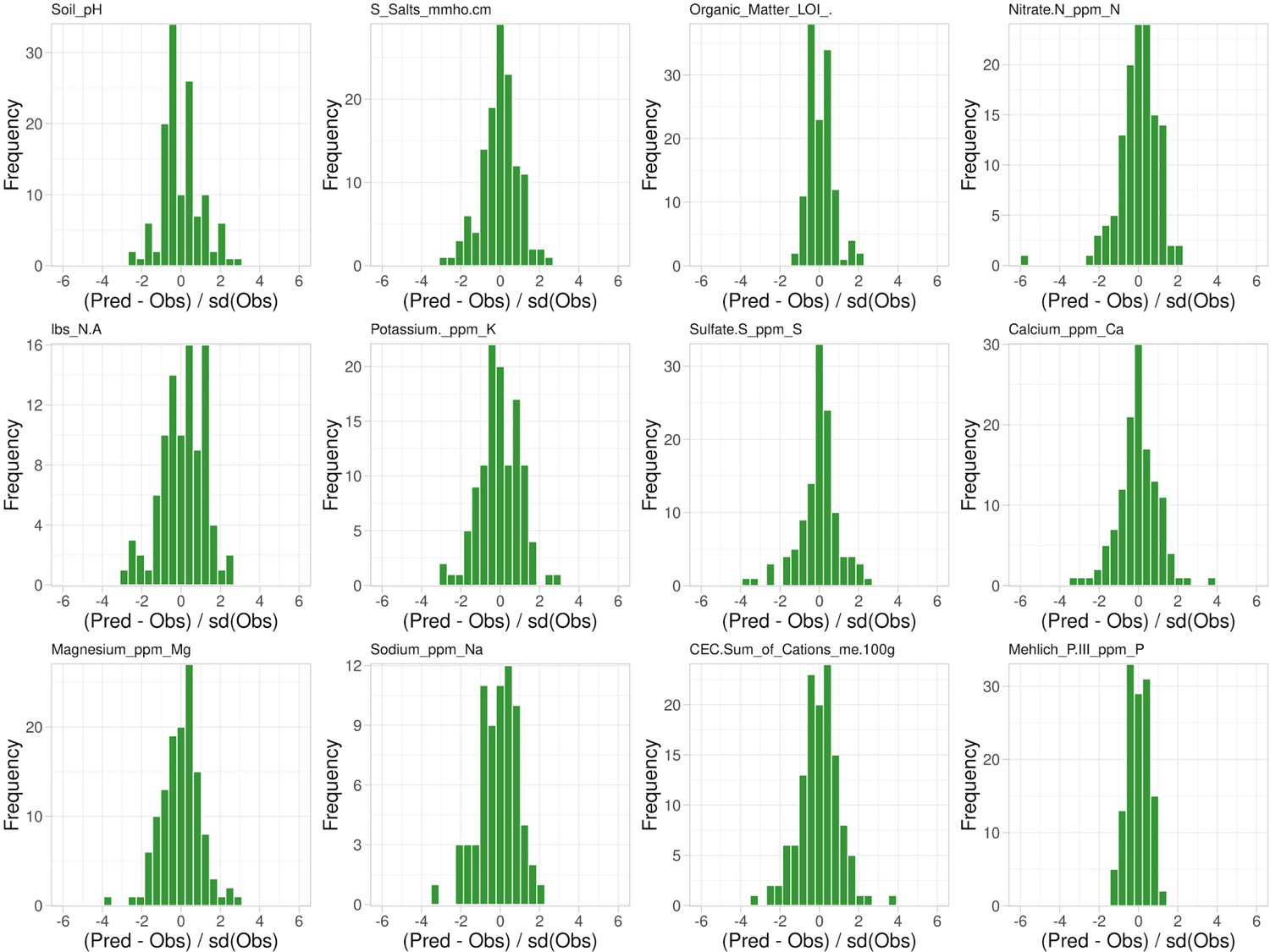
Leave-one-out cross-validation of soil property observations.
Shown is the difference between the predicted and the observed values for each sample normalized to the standard deviation of the observations, x-axis, and their respective frequency, y-axis.
Figure 1—figure supplement 2
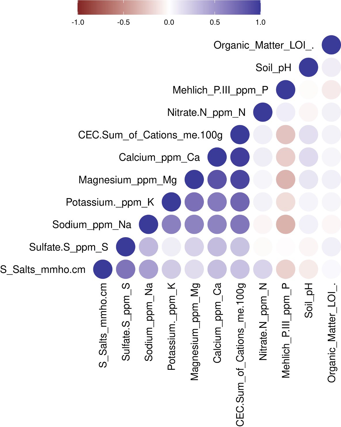
Pearson correlations between all pairwise soil properties.
Negative correlations are depicted as shades of red, and positive correlations are depicted as blue. Soil properties are ordered by hierarchical clustering based on Euclidean distance and complete agglomeration.
Figure 2 with 1 supplement
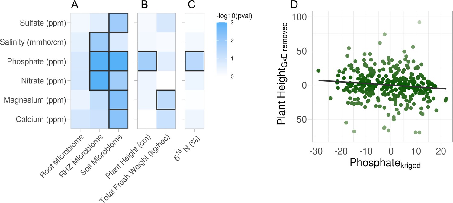
Association of soil property variations with multiple phenotypes.
Six soil properties were assessed for effect on root microbiome and plant phenotypes using permutation ANOVA. Cells are colored by −log10 p value of the effect. (A) Effect of each soil property on microbiome beta diversity from three root compartments: root (endosphere), RHZ (rhizosphere), and soil (bulk soil), while constraining on genotype and treatment. Effect of each soil nutrient on the height and weight (B) and leaf δ15N (C) using type III sum of squares while including treatment, genotype, and interaction as additional fixed effects. (D) Example effect of kriged phosphate, x-axis, on plant height, adjusted for genotype and treatment, y-axis.
Figure 2—figure supplement 1
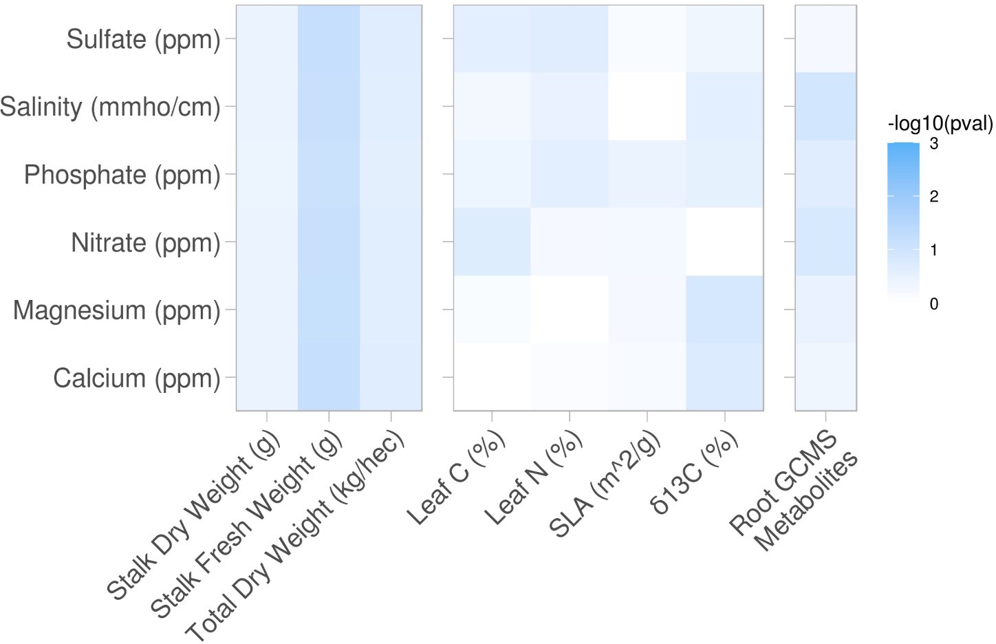
Same analysis as Figure 2A-C, but here are shown the phenotypes that did not demonstrate soil property associations.
Figure 3
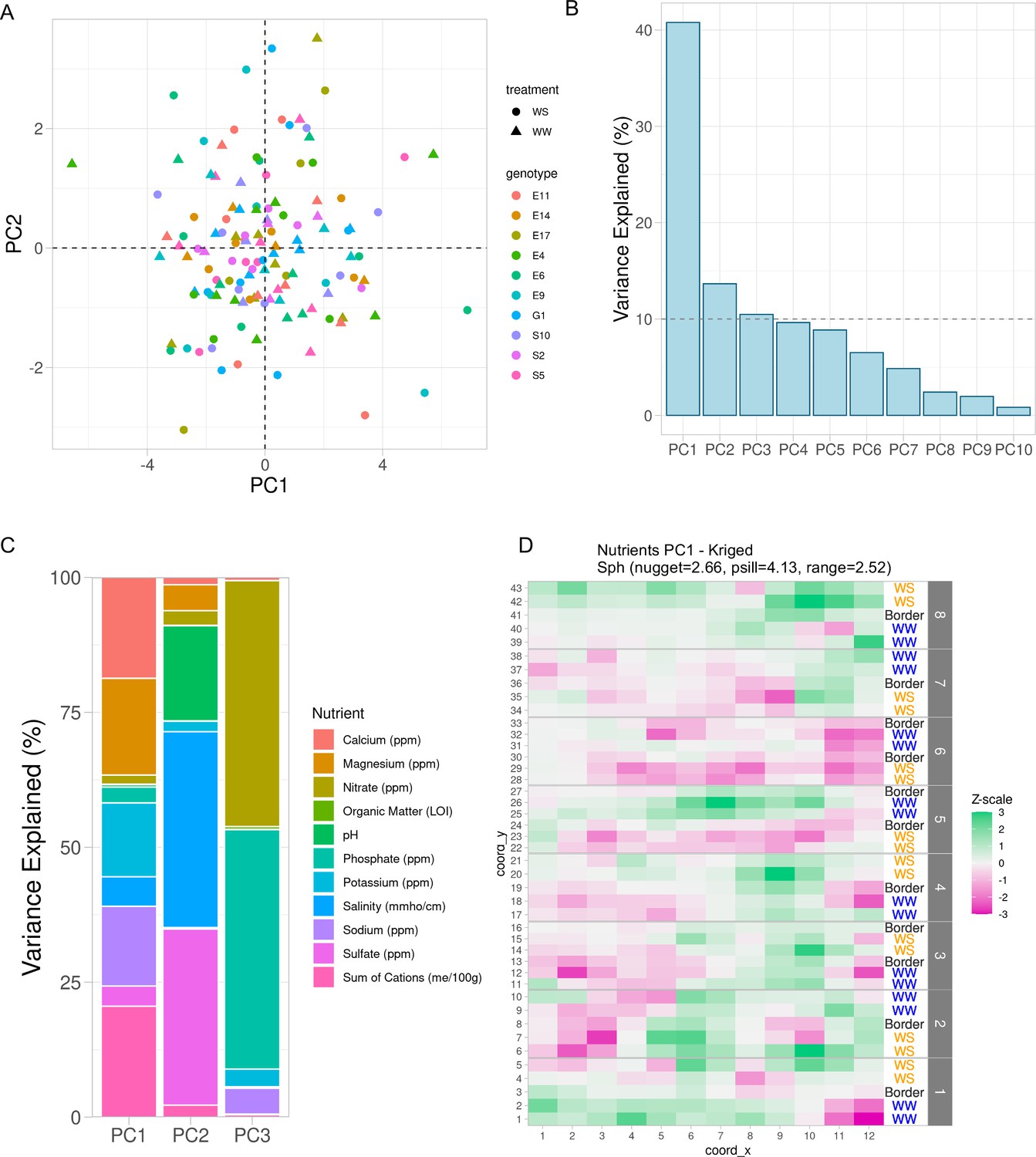
Variation in soil properties can be collapsed into principal components.
(A) First two principal components of soil property residuals as x- and y-axis, respectively, colored by genotype and shaped by treatment. (B) Scree plot of the first 10 principal components. Shown is the percent variance explained of the total property variance by each component. Dashed line is at 10% variance explained. (C) For the first three components, colored is the contribution of each soil property to its respective variance explained within each component. (D) Spatial distribution of kriged PC1. Each cell colored by scaling the values to unit variance. Variogram fit with nugget, partial sill, and range displayed.
Figure 4 with 2 supplements

Accounting for influence from soil property variance within microbiome data reveals plant phenotypes that correlate with microbe abundance.
(A) Principal component analysis on the combined raw and residual microbiome tables. Shown are the first two components with their respective variance explained. Samples are colored by tissue type and shaped by original or residual values. Gray points are the centers of each respective cluster, and gray lines connect the centers of each cluster. (B) Partial correlations of experimental design variables in each microbiome compartment’s composition before and after principal component regression. (C) Observed plant height values, x-axis, and the change in that value as a result of the adjustment, y-axis. (D) Similar to C, shown are the fresh weight values and their respective changes. In both C and D, horizontal green dashed lines represent the 95% confidence interval for the change in observation. Light gray dots are within the interval, and dark gray dots are outside of the interval. (E) Partial correlations of experimental design variables in leaf δ15N before and after principal component regression. (F, G) For only water-stressed samples and only the soil microbiome, plant height, y-axis, and operational taxonomic unit (OTU) abundance of Microvirga, x-axis, before and after principal component regression. Shown in G, is the fit of a change-point model where the red line is no change before threshold, the vertical dashed line, and the blue line is a linear fit after the threshold.
Figure 4—figure supplement 1
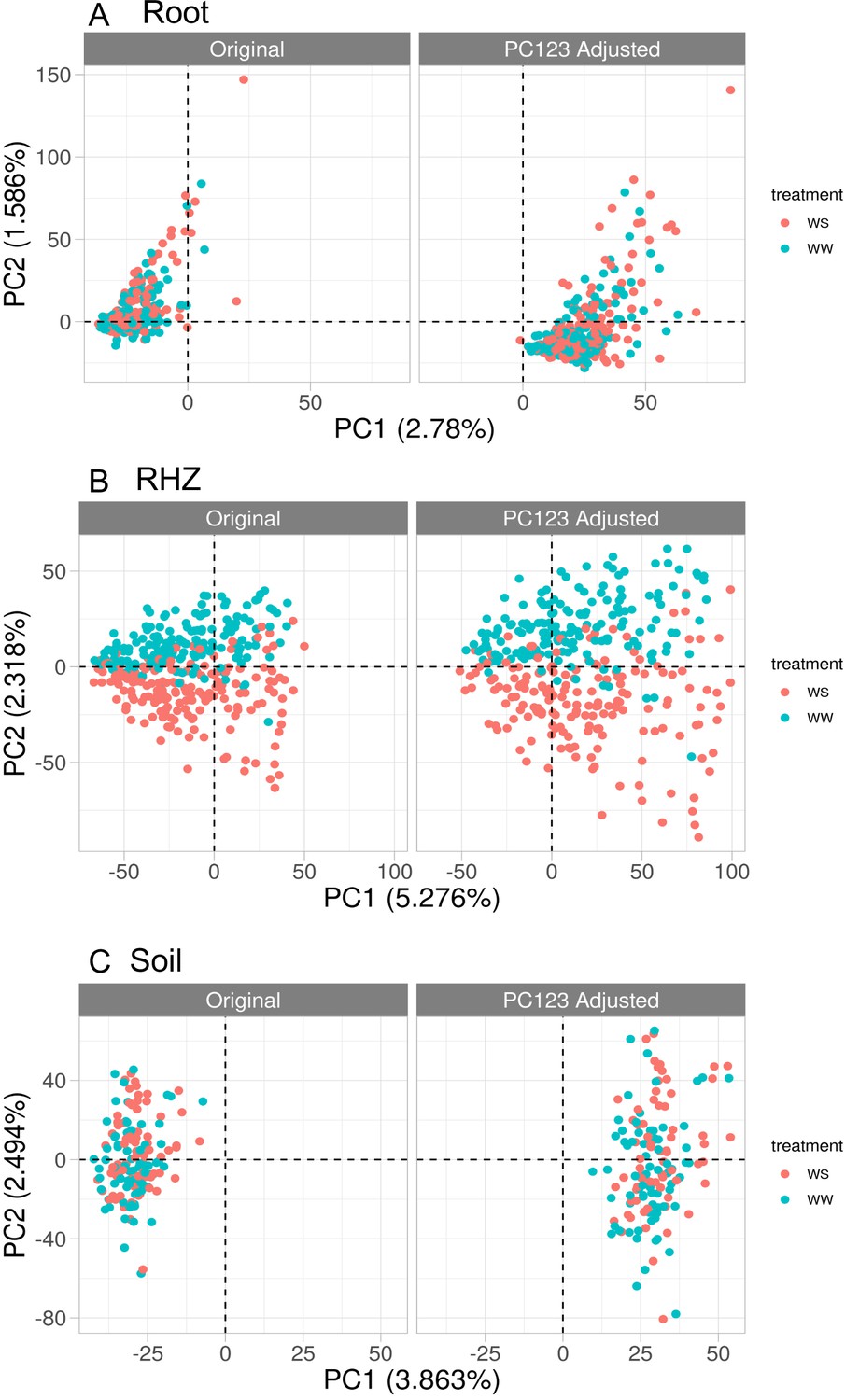
Principal component analysis on the root (A), rhizosphere (B), and soil (C) samples using the combined raw and residual microbiome tables.
Left panel uses the original counts and right uses adjusted counts (see Methods: Principal component regression). Each panel has colors corresponding to the treatment for each sample.
Figure 4—figure supplement 2
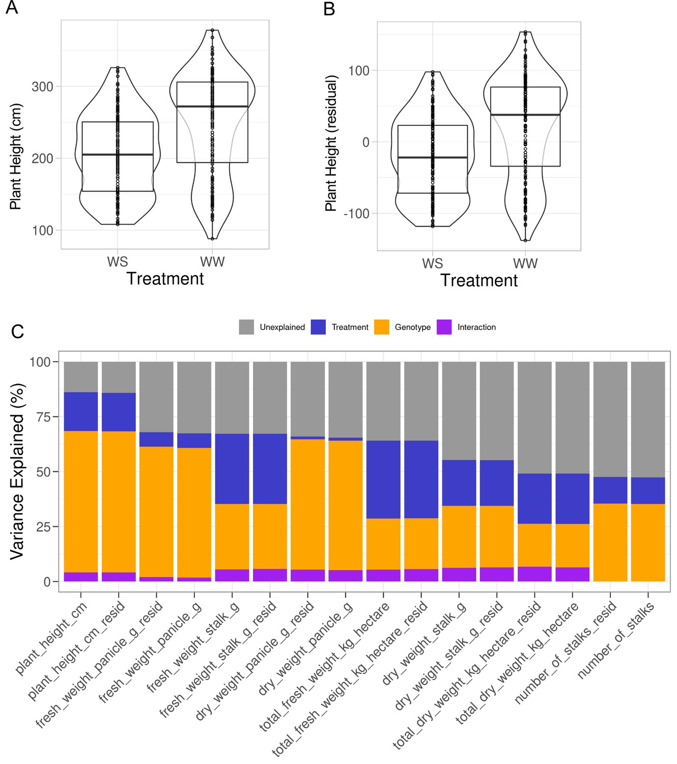
Effect of applying principal component regression on plant morphology.
(A) Boxplots, overlaying violin plots, of plant height, y-axis, against the watering treatments (WS: drought, WW: well-watered), x-axis. (B) Same as A, but displaying the residuals of plant height, y-axis, from principal component regression model using dimension reduced soil properties as covariates. See Qi et al., 2022 for additional details and analysis on these data. (C) Variance components, y-axis, of each harvest trait measured, x-axis, for both original data and adjusted data (_resid).
Tables
Table 1
Shown are sum-of-square errors for each soil property (columns) and each spatial model tested (rows).
Cells that have asterisks are those models that have minimal errors and are chosen to be the best-fit model for kriging for the respective soil property.
| Salinity | Nitrate | Sulfate | Calcium | Magnesium | Phosphate | |
|---|---|---|---|---|---|---|
| Nugget only | 1.92115E−05 | 203.668 | 10645.6 | 833211000 | 2261360 | 149,688 |
| Exponential | 1.1769E−06 | 41.2651 | 1909.53 | 17886300000 | 65136300 | 27556.2 |
| Spherical | 2.03099E−06 | 25.5247 | 2058.42 | 244155000* | 1038010* | 32351.9 |
| Gaussian | 2.16269E−06 | 22.3183* | 289,060 | 17669600000 | 64365000 | 100,531 |
| Matern | 0.00000113273* | 23.0069 | 1682.03* | 266373000 | 1087980 | 18961.6 |
| Stein’s Matern | 1.13273E−06 | 23.0069 | 290,357 | 17886300000 | 65136300 | 18827.8* |
Table 2
Shown for each soil property that exhibits significant spatial distribution (see Methods: Statistical testing for evidence of spatial structure) (first column) is the interaction effect with the different microbiome tissue compartments on the overall microbiome composition (p value <0.05 indicates significant interaction, PERMANOVA from model: Composition ~ Property:Compartment).
| Soil property | p value |
|---|---|
| Sulfate (ppm) | 0.24 |
| Salinity (mmho/cm) | 0.011 |
| Phosphate (ppm) | 0.001 |
| Nitrate (ppm) | 0.001 |
| Magnesium (ppm) | 0.003 |
| Calcium (ppm) | 0.005 |
Table 3
Shown for each microbiome compartment are the number of operational taxonomic units (OTUs) that showed significant association (p value <0.05) in their abundance to the respective phenotype, either positive or negative, both before (original) and after (PC123 Adj) principal component regression.
The intersection column shows the number of OTUs shared between these two sets of counts.
| Compartment | Phenotype | Original | PC123 Adj | Intersection |
|---|---|---|---|---|
| Soil | Dry weight | 7950 | 445 | 155 |
| RHZ | Dry weight | 5619 | 897 | 333 |
| Root | Dry weight | 3320 | 231 | 96 |
| Soil | Plant height | 7991 | 342 | 137 |
| RHZ | Plant height | 5614 | 854 | 329 |
| Root | Plant height | 3397 | 245 | 97 |
Additional files
Download links
A two-part list of links to download the article, or parts of the article, in various formats.
Downloads (link to download the article as PDF)
Open citations (links to open the citations from this article in various online reference manager services)
Cite this article (links to download the citations from this article in formats compatible with various reference manager tools)
Increased signal-to-noise ratios within experimental field trials by regressing spatially distributed soil properties as principal components
eLife 11:e70056.
https://doi.org/10.7554/eLife.70056


