A unifying mechanism governing inter-brain neural relationship during social interactions
Figures
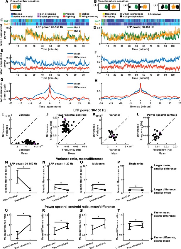
Relative magnitudes and timescales of the inter-brain difference and mean components.
(A) In each one-chamber session, two bats freely interacted with each other while neural activity was wirelessly recorded simultaneously from their frontal cortices. (B) In each two-chambers session, the same bats from the one-chamber sessions freely behaved in separate, identical chambers, while neural activity continued to be simultaneously and wirelessly recorded from their frontal cortices. Two-chambers sessions included three conditions: (1) two bats each freely behaving in isolation; (2) two bats each freely behaving while listening to identical auditory stimuli; (3) two bats each freely behaving and interacting with a different partner in separate chambers. (C)-(D) Mean normalized LFP power in the 30–150 Hz band (Materials and methods), averaged across all channels for each bat, on an example one-chamber session (C) and an example two-chambers session (D). Shown above are the behaviors of the two bats as a function of time, which were manually annotated frame-by-frame from recorded video. The example two-chambers session was of the third type illustrated in (B). (E) The neural activity of the two bats from (C) after a change of basis, showing the mean and difference between bats. At a given time , the mean and difference components are defined as and , respectively, where and are respectively the neural activity of bat 1 and bat 2 plotted in (C). Note that the mean component had a large variance, whereas the difference component had a small variance, hovering around zero. (F) Same as (E), but for the example session from (D). Note that the variances are more comparable between the mean and difference components. (G) Autocorrelations (peak-normalized) of the mean and difference components shown in (E). The autocorrelations were computed after subtracting from each time series its average over time. Note that the difference component varied on faster timescales than the mean component. (H) Same as (G), but for the example session from (D). Note that the timescales are more comparable between the mean and difference components. (I)-(J) Variance (I) and power spectral centroid (J) of mean normalized 30–150 Hz LFP power, for the mean and difference components. Each dot is a single one-chamber session (the purple dot is the session shown in (C), (E), and (G)). Variance quantifies activity magnitude, and power spectral centroid quantifies timescale (higher centroids mean faster timescales). Note that, on every one-chamber session, the difference component was smaller and faster than the mean component. The dotted lines are unity. Note that the power spectral centroid was calculated from time series of mean normalized LFP power (e.g., as plotted in (E)), not from time series of LFP itself. (K)-(L) Same as (I)-(J), but for two-chambers sessions. The purple dot is the session shown in (D), (F), and (H). The mean and difference components have comparable magnitudes and timescales in the two-chambers sessions. (M)-(P) The average variance ratio (mean component variance divided by difference component variance) for mean normalized 30–150 Hz LFP power (M), mean normalized 1–29 Hz LFP power (N), multiunits (O), and single units (P). The averages were taken across sessions for LFP power, and across unit pairs (pooled from all sessions) for multiunits and single units. Error bars denote standard deviations. *, p < 0.05, Wilcoxon rank sum test. (Q)-(T) Same as (M)-(P), but for average power spectral centroid ratio (mean component centroid divided by difference component centroid). Note that, for all four neural signals, the difference component was smaller and faster than the mean component on one-chamber sessions. See Figure 1—figure supplements 2–4 for examples and detailed results for 1–29 Hz LFP power, multiunits, and single units.
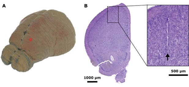
Neural recording location.
(A) An example bat brain reconstructed from block-face imaging, with the electrode location in frontal cortex indicated by a red circle. (B) Left: an example Nissl-stained coronal section, at the location of the red circle in (A), showing a tetrode track (dashed box). Right: zoomed-in view showing the tetrode track (arrow).
© 2019, Elsevier. Figure 1—figure supplement 1 is reprinted from Figure S1 from Zhang and Yartsev, 2019, with permission from Elsevier. It is not covered by the CC-BY 4.0 license and further reproduction of this panel would need permission from the copyright holder.
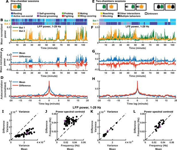
Inter-brain difference and mean components: 1–29 Hz LFP power.
(A) One-chamber sessions: simultaneous neural recording from pairs of bats engaged in natural social interactions. (B) Mean normalized LFP power in the 1–29 Hz band (Materials and methods), averaged across all channels for each bat, on an example one-chamber session. Shown above are the annotated behaviors. (C) The mean and difference components of the activity of the two bats shown in (B). (D) Autocorrelations (peak-normalized) of the mean and difference activity components shown in (C). The autocorrelations were computed after subtracting from each time series its average over time. Note that the difference component varied on faster timescales than the mean component. (E) Two-chambers sessions: simultaneous neural recording from the same bats from the one-chamber sessions freely behaving in separate, identical chambers. (F)-(H) Same as (B)-(D), but for an example two-chambers session. (I)-(J) Variance (I) and power spectral centroid (J) of mean normalized 1–29 Hz LFP power, for the mean and difference components. Each dot is one one-chamber session (the purple dot is the session shown in (B)-(D)). Variance quantifies activity magnitude, and power spectral centroid quantifies timescale (higher centroids mean faster timescales). Note that, on one-chamber sessions, the difference component tends to be smaller and faster than the mean component. The dotted lines are unity. Note that the power spectral centroid was calculated from time series of mean normalized LFP power (e.g. as plotted in (C)), not from time series of LFP itself. (K)-(L) Same as (I)-(J), but for two-chambers sessions. The purple dot is the session shown in (F)-(H). The mean and difference components have comparable magnitudes and timescales on the two-chambers sessions.
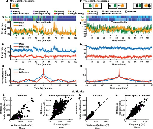
Inter-brain difference and mean components: multiunit activity.
(A) One-chamber sessions: simultaneous neural recording from pairs of bats engaged in natural social interactions. (B) Activity of two multiunits, one from each brain, on an example one-chamber session. Shown above are the annotated behaviors. (C) The mean and difference components of the activity of the two bats shown in (B). (D) Autocorrelations (peak-normalized) of the mean and difference activity components shown in (C). The autocorrelations were computed after subtracting from each time series its average over time. Note that the difference component varied on faster timescales than the mean component. (E) Two-chambers sessions: simultaneous neural recording from the same bats from the one-chamber sessions freely behaving in separate, identical chambers. (F)-(H) Same as (B)-(D), but for an example two-chambers session. (I)-(J) Variance (I) and power spectral centroid (J) of multiunit activity, for the mean and difference components. Each dot is one pair of multiunits (one from each brain) from one-chamber sessions (the purple dot is the pair shown in (B)-(D)). Variance quantifies activity magnitude, and power spectral centroid quantifies timescale (higher centroids mean faster timescales). Note that, on one-chamber sessions, the difference component tends to be smaller and faster than the mean component. The dotted lines are unity. (K)-(L) Same as (I)-(J), but for two-chambers sessions. The purple dot is the pair of multiunits shown in (F)-(H). The mean and difference components have comparable magnitudes and timescales on the two-chambers sessions.
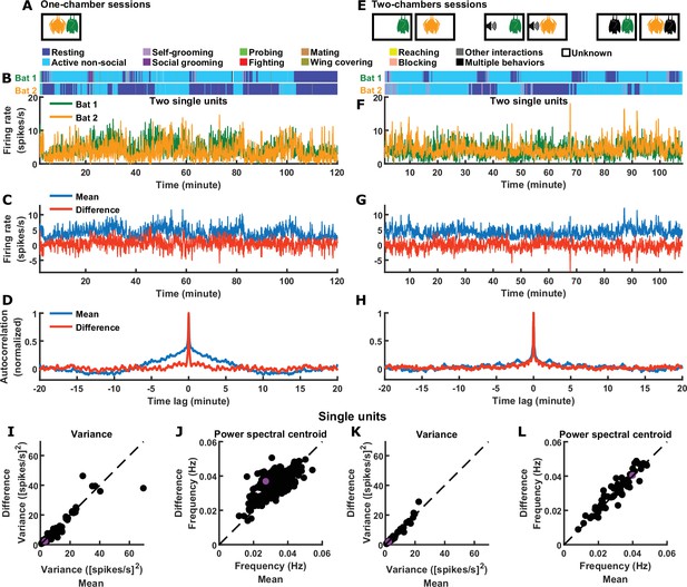
Inter-brain difference and mean components: single unit activity.
(A) One-chamber sessions: simultaneous neural recording from pairs of bats engaged in natural social interactions. (B) Activity of two single units, one from each brain, on an example one-chamber session. Shown above are the annotated behaviors. (C) The mean and difference components of the activity of the two bats shown in (B). (D) Autocorrelations (peak-normalized) of the mean and difference activity components shown in (C). The autocorrelations were computed after subtracting from each time series its average over time. (E) Two-chambers sessions: simultaneous neural recording from the same bats from the one-chamber sessions freely behaving in separate, identical chambers. (F)-(H) Same as (B)-(D), but for an example two-chambers session. (I)-(J) Variance (I) and power spectral centroid (J) of single unit activity, for the mean and difference components. Each dot is one pair of single units (one from each brain) from one-chamber sessions (the purple dot is the pair shown in (B)-(D)). Variance quantifies activity magnitude, and power spectral centroid quantifies timescale (higher centroids mean faster timescales). The dotted lines are unity. (K)-(L) Same as (I)-(J), but for two-chambers sessions. The purple dot is the pair of single units shown in (F)-(H).
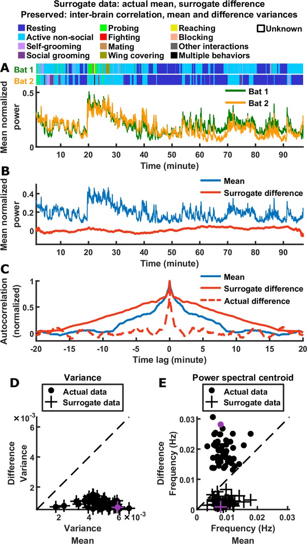
Relative timescales of the difference and mean components are not determined by their relative magnitudes or levels of inter-brain correlation.
(A) Surrogate data generated from the actual data shown in Figure 1C, by combining the actual mean component with a surrogate difference component (Materials and methods). The surrogate was tailored such that the difference component variance and inter-brain correlation of the original experimental data were preserved (the mean component variance was also preserved since the actual mean component was used in the surrogate data). Shown above are the actual behaviors of the two bats replotted from Figure 1C. (B) The surrogate data from (A) plotted as the activity of its mean and difference components. The mean here is identical to the actual mean in Figure 1E, while the difference here has the same variance as the actual difference in Figure 1E, but with slower timescales. (C) The autocorrelations (peak-normalized) of the mean and difference components shown in (B) and of the actual difference component shown in Figure 1E. The autocorrelations were computed after subtracting from each time series its average over time. Note that for the surrogate data, the difference was slower than the mean, the opposite of what was observed experimentally. (D)-(E) Variance (D) and power spectral centroid (E) of mean normalized 30–150 Hz LFP power, for the mean and difference components of the actual data and surrogate data. Each dot is actual data from a single one-chamber session (replotted from Figure 1I–J), and each plus is surrogate data generated from the actual data of a single one-chamber session (purple dots and pluses denote the example session shown in Figure 1C and (A)-(C)). The dotted lines are unity. The surrogate data preserve the actual inter-brain correlations (Materials and methods), as well as the variances of the actual mean and difference components (pluses in (D) are at the same positions as the dots), but have slower difference components than mean components (pluses below the unity line in (E)).
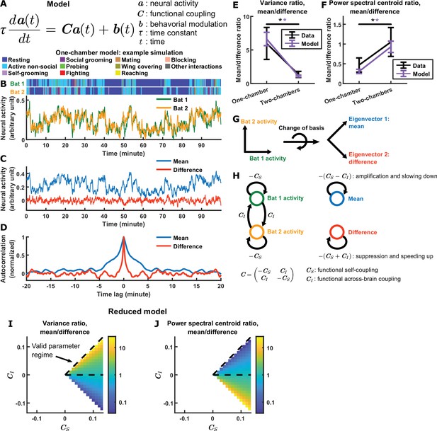
Model explains relationship between difference and mean.
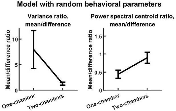
(A) The evolving neural activity of two bats are modeled by a linear differential equation. is the activity of bat 1 and bat 2 at time . is the functional coupling matrix, where is the strength of functional self-coupling and is the strength of functional across-brain coupling (note that functional across-brain coupling obviously should not be interpreted as direct coupling via actual neural connections). is the modulation of each bat’s activity by its behaviors, where the behaviors are simulated using Markov chains. See Materials and methods for details on the model and for the values of the parameters. (B) Simulated neural activity and behaviors from an example one-chamber simulation. (C) The simulated activity from (B) plotted as the activity of its mean and difference components. Note the smaller magnitude of the difference compared to the mean. (D) The autocorrelations (peak-normalized) of the mean and difference components shown in (C). The autocorrelations were computed after subtracting from each time series its average over time. Note that the difference varied on faster timescales than the mean. (E)-(F) The average variance ratio (E; mean component variance divided by difference component variance) and average power spectral centroid ratio (F; mean component centroid divided by difference component centroid), for model simulations (purple) or mean normalized 30–150 Hz LFP power from the data (black). The averages were taken across simulations for the model, and across sessions for the data. Error bars denote standard deviations. *, p < 0.05, Wilcoxon rank sum test. (G)-(H) Model mechanism. See Materials and methods for details. (G) Schematic illustrating a change of basis for representing the model. The model describes the neural activity of two bats evolving in a 2D space. Activity in this space can be represented using any choice of axes. The equation in (A) assumes the axes illustrated on the left, where each axis is the neural activity of one bat. After a rotation of 45 degrees, the axes now represent the mean and difference components (illustrated on the right), which are also the eigenvectors of the functional coupling matrix . (H) The neural activity variables of the two bats are coupled to each other (left). Changing to the eigenvector basis transforms them into uncoupled variables: the mean and difference components (right). The mean and difference components each provides feedback onto itself, with feedback strengths being the eigenvalues of , which depend on the functional across-brain coupling . In the one-chamber model, , so functional across-brain coupling amplifies and slows down the mean component through positive feedback, and suppresses and speeds up the difference component through negative feedback. (I)-(J) The dependence of variance ratio (I) and power spectral centroid ratio (J) on the coupling strength parameters, for a reduced model where the behavioral modulation for the mean and difference components have identical, flat power spectra. The variance ratio and centroid ratio are approximately and , respectively; thus, the parameter regime that qualitatively reproduces experimental observations is the regime of positive functional across-brain coupling (delimited by dashed lines). The white spaces are regions of the parameter space where the model is unstable. Note that the color maps are in log scale. See Materials and methods for details.
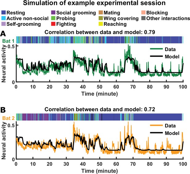
Comparing actual and simulated neural activity as a function of time.
(A)-(B) Neural activity (mean normalized LFP power in the 30–150 Hz band) on an example experimental session is compared to model activity simulated using actual behaviors from that session (instead of behaviors generated using a Markov chain). The activity and behavior of bats 1 and 2 are plotted in (A) and (B), respectively. The correlations between the actual and simulated activity are indicated above each plot (the average correlation over all sessions and bats is 0.72, with a standard deviation of 0.10). See Materials and methods for details.
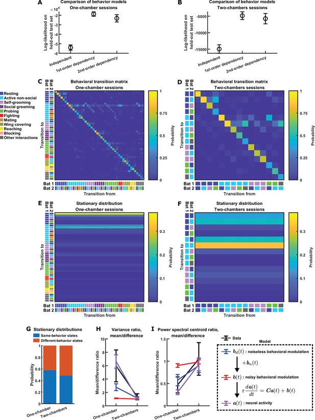
Behavior models.
(A)-(B) Comparison of three models for bat behavior: (1) a model where the behavioral state at any time point is independent from other time points (‘Independent’); (2) a first-order Markov chain (‘first-order dependency’); (3) a second-order Markov chain (‘second-order dependency’). Plotted are log-likelihoods under the three models on test sets not used for model fitting, for the one-chamber (A) and two-chambers (B) sessions. Error bars denote standard deviation across 100 random splits of the data into training and test sets. The first-order Markov chain had the highest likelihood on average and were chosen as our behavior model (C)-(F). See Materials and methods for details. (C)-(D) Empirical behavioral transition frequency matrix for the one-chamber (C) and two-chambers (D) sessions, used to simulate behaviors using first-order Markov chains (Materials and methods). A behavioral state consists of the behaviors of both bats: for exmple one state could be ‘bat 1 resting, bat 2 self-grooming’. Each matrix shows the frequencies of transition from one state at a given time to another state after a passage of 2.5 s (the time step size of the Markov chains): the color of the matrix element at row i and column j denotes the frequency of transitions from state j to state i. The states are labeled by color to the left and bottom of the matrices. Here the diagonal elements (self-transitions) are larger than the off-diagonal elements (transitions between states) because of the small time step size of the Markov chain. The transition frequencies were calculated after pooling the behavioral data from all one-chamber (C) or two-chambers (D) sessions. (E) Multi-step transition matrix showing the transition probability from one state at a given time to another state after a passage of 5 min, in the one-chamber model. This matrix was obtained by raising the single-step transition matrix in (C) to the 120th power. Note that the columns of the multi-step transition matrix are approximately identical, showing that the Markov chain approaches the stationary distribution represented by the columns within ~5 minutes, that is, the distribution of states no longer changes with time ~5 min into a simulated session. (F) Same as (E) but for the two-chambers model. (G) The probability of same-behavior states and different-behavior states in the stationary distributions of the one-chamber and two-chambers models. A same-behavior state is defined as a state where the two bats engage in the same behavior, and a different-behavior state is one where the two bats engage in different behaviors. In the stationary distribution of the two-chambers Markov chain, same-behavior states (probability: 0.49) are about equally likely as different-behavior states. In the stationary distribution of the one-chamber Markov chain, same-behavior states (probability: 0.58) are somewhat more likely than different-behavior states. (H)-(I) The average variance ratio (H; mean component variance divided by difference component variance) and average power spectral centroid ratio (I; mean component centroid divided by difference component centroid), for variables from the model (blue, red, and purple) and for mean normalized 30–150 Hz LFP power from the data (black). The model variables include noiseless behavioral modulation (blue), noisy behavioral modulation (red), and neural activity (purple); the relationships between the variables are illustrated in the dashed box (Materials and methods). Note that in the one-chamber model, the noiseless behavioral modulation of the mean component is larger and slower than that of the difference component (blue). Behavioral modulation noise decreases the differential modulation of the mean and difference components (red). However, even when the noise strongly reduces differential behavioral modulation of the mean and difference components, the experimentally observed levels of relative activity magnitudes and timescales can still result (purple), due to functional across-brain coupling (Figure 3G–H and Materials and methods). The plotted averages were taken across simulations for the model, and across sessions for the data. The data (black) and simulated activity (purple) are replotted from Figure 3E–F. Error bars denote standard deviations. See Materials and methods for details.
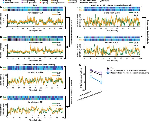
Comparing models with and without functional across-brain coupling.
(A) Mean normalized LFP power in the 30–150 Hz band, averaged across all channels for each bat, on an example one-chamber session. Shown above are the annotated behaviors. Note that the activity of the two bats are highly correlated (correlation coefficient indicated above the activity traces). (B) The same data as in (A), after removing all time periods of coordinated behavior (i.e., time periods when both bats engaged in the same behavior). Inter-brain correlation was re-calculated and indicated above the activity traces. Note that the inter-brain correlation is lower than in (A), but still highly positive. (C)-(D) Same as (A)-(B), but for simulated neural activity and behaviors from an example one-chamber simulation of our main model. Note that inter-brain correlation remained after removing time periods of coordinated behavior, reproducing the experimental result. (E)-(F) Same as (C)-(D), but simulated without functional across-brain coupling. Specifically, the same simulated behavior and behavioral modulation was used as in (C)-(D); the difference from (C)-(D) is that the strength of functional across-brain coupling was set to 0. Note that inter-brain correlation disappeared after removing time periods of coordinated behavior, unlike the experimental result. (G) Inter-brain correlation over entire sessions or after removing coordinated behavior, for data (black; mean normalized LFP power in the 30–150 Hz band), the main model (purple; with functional across-brain coupling), and the model without functional across-brain coupling (blue). The simulations of the two models were done in pairs: each simulation of the model without functional across-brain coupling used the same behavioral modulation (including behavioral modulation noise) as one simulation of the main model, as done in (C)-(F). Plotted are averages (± standard deviation) across experimental sessions or simulations. Note that functional across-brain coupling is required in the model to reproduce persisting inter-brain correlation after the removal of coordinated behaviors. See Materials and methods for details.
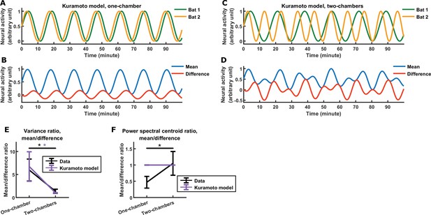
A Kuramoto model of the inter-brain relationship.
The Kuramoto model uses an alternative form of functional across-brain coupling compared to our main model of Figure 3. In the Kuramoto model, the neural activity of the interacting bats are abstracted as oscillators whose phases are dynamically coupled depending on their phase difference. See Materials and methods for details. (A)-(B) Example simulation of the one-chamber Kuramoto model, shown as the activity of the two bats (A) and as the mean and difference between bats (B). The model exhibits inter-brain correlation, as well as a larger magnitude for the mean component compared to the difference component. However, the difference and mean components have the same timescale in this model (note that the difference and mean undergo the same number of oscillations per unit time). (C)-(D) Same as (A)-(B), but for the two-chambers Kuramoto model. Here, the difference and mean components have similar magnitudes and timescales. (E)-(F) The average variance ratio (E; mean component variance divided by difference component variance) and average power spectral centroid ratio (F; mean component centroid divided by difference component centroid), for Kuramoto model simulations (purple) or mean normalized 30–150 Hz LFP power from the data (black). The averages were taken across simulations for the model, and across sessions for the data. Note that the Kuramoto model reproduces the relative magnitudes, but not the relative timescales, from the data. The results for data (black) are replotted from Figure 3E–F. Error bars denote standard deviations. *, p < 0.05, Wilcoxon rank sum test.
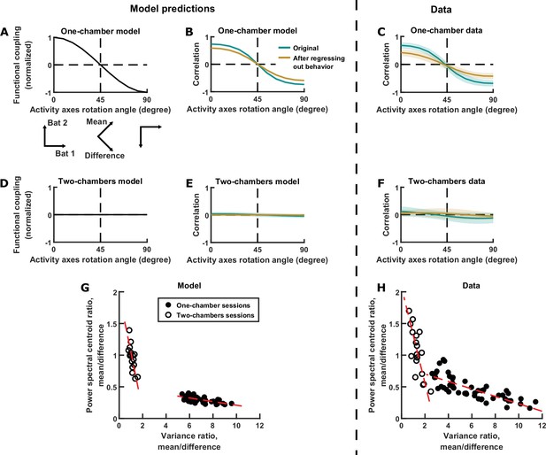
Testing model predictions.
(A), (B), (D), (E), and (G) show model results and predictions, and (C), (F), and (H) show the corresponding data. (A) The neural activity of two bats can be represented in a 2D space, using any choice of axes orientation for the space. In our model, the axes orientation determines the strength of coupling between the activity variables represented by the axes. Here, functional coupling between the activity variables in the one-chamber model is plotted against the axes orientation defining the activity variables. When the activity variables correspond to the activity of each bat (0° rotation), functional coupling is at its positive maximum. Functional coupling decreases as the axes rotate, becoming zero when the activity variables correspond to the mean and difference components (45° rotation). Three orientations of the axes are illustrated below the plot. The plotted functional coupling was normalized by the functional coupling at 0° rotation. (B) Correlation between the activity variables in the one-chamber model, plotted against the orientation of the axes of the activity space that defines the activity variables. Correlations were shown both before (teal) and after (brown) regressing out the behaviors of both bats from each activity variable. Shading indicates standard deviation across simulations. Note that the shape of the correlation curves mirrors that of functional coupling shown in (A), and that regressing out behaviors changes the magnitude, but not the shape of the correlation curve. (C) Same as (B), but for data from one-chamber sessions. Shading indicates standard deviation across sessions. Note that the data confirms the model predictions from (B). (D)-(F) Same as (A)-(C), but for the two-chambers model and data. Note that the data again confirms model predictions. (G) Scatter plot of power spectral centroid ratio (mean component centroid divided by difference component centroid) vs. variance ratio (mean component variance divided by difference component variance). Each circle is a simulation (filled: one-chamber model; open: two-chambers model). Red dashed lines are total least squares regression lines. Note that the model predicts linear relationships between the variance ratio and centroid ratio. See Figure 5—figure supplement 1 and Materials and methods for detailed analysis of these relationships. (H) Same as (G), but for the data. Note that the prediction from (G) is confirmed by the data.
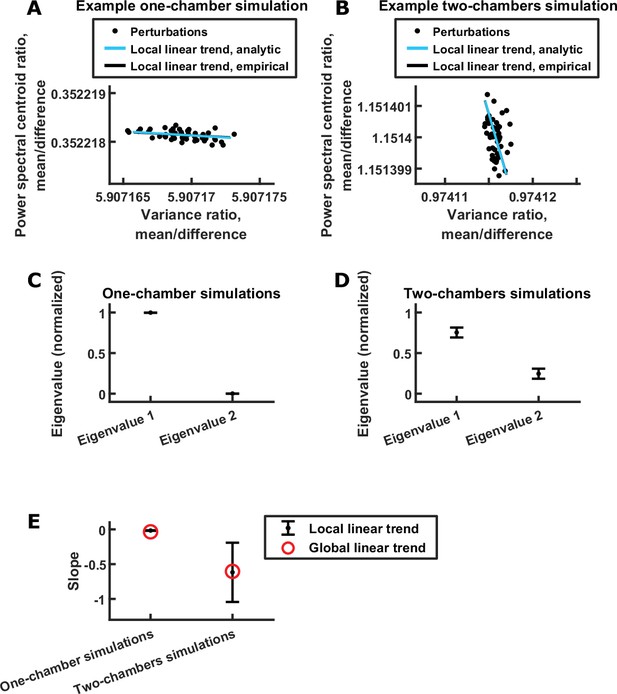
Analysis of linear relationship between power spectral centroid ratio and variance ratio.
(A) Scatter plot of power spectral centroid ratio (mean component centroid divided by difference component centroid) vs. variance ratio (mean component variance divided by difference component variance), after small random perturbations to the behavioral modulation for a single one-chamber simulation. Each dot is the result of one random perturbation. The blue line is the analytic estimated direction of the linear trend (Materials and methods), and the black line is the empirical direction of the linear trend calculated from 1,000 random perturbations (of which a random subset of 50 are plotted, for clarity). The black line is not visible because it is overlapped by the blue line. Note that a clear linear trend is present despite behavioral modulation being randomly perturbed. (B) Same as (A) but for a two-chambers simulation. (C) For a given one-chamber simulation, we estimated the eigenvalues of the covariance matrix of power spectral centroid ratio and variance ratio resulting from random perturbations to the behavioral modulation of that simulation (Materials and methods). Each eigenvalue was then normalized by the sum of the eigenvalues. Plotted are the averages (± standard deviation) of the normalized eigenvalues across simulations, with eigenvalue one being the larger eigenvalue from each simulation. Note that one eigenvalue was much larger than the other across simulations, indicating a linear trend. (D) Same as (C) but for two-chambers simulations. Note that, again, one eigenvalue tended to be larger than the other. (E) The slopes of the global (red) and local (black) linear relationships between power spectral centroid ratio and variance ratio. The global slopes are the slopes of the linear fit across simulations (like the red dashed lines in Figure 5G, but for 100 simulations). The local slopes are the slopes of the blue lines in (A)-(B): for each simulation, the local slope was calculated from the leading eigenvector of the covariance matrix of power spectral centroid ratio and variance ratio resulting from random perturbations (Materials and methods). The average local slopes across simulations were then plotted (error bars denote standard deviations). Note that the local slopes, which are not influenced by systematic variations of behavioral modulation across simulations, are consistent with the global slopes.
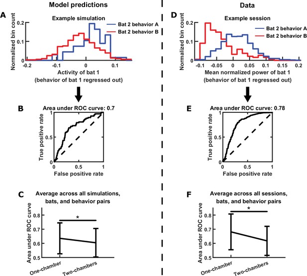
Testing further model predictions.
(A)-(C) show model results and predictions, and (D)-(F) show the corresponding data. (A) Distributions of the neural activity of bat 1 conditioned on the behavior of bat 2. Bat 1’s behavior has been regressed out of its neural activity. Two distributions are shown from an example simulation, for two example behaviors by bat 2 (behavior A: probing; behavior B: resting). Note that bat 1’s activity encodes bat 2’s behavior independently of its own behavior. (B) The extent to which bat 1’s activity encodes the two behaviors of bat 2 in the example from (A) is quantified using an ROC curve, which illustrates the discriminability of the two distributions from (A). The area under the ROC curve is indicated above the plot (larger area indicates better discriminability). (C) Area under the ROC curve is averaged across all simulations, bats, and behavior pairs, separately for one-chamber simulations and two-chambers simulations. When using one bat’s activity to discriminate the other bat’s behavior, discriminability is significantly higher in one-chamber simulations. Error bars denote standard deviations. *, p < 0.05, Wilcoxon rank sum test. (D)-(F) Same as (A)-(C), but for mean normalized 30–150 Hz LFP power from the data. For the example in (D), behaviors A and B are active non-social and social grooming, respectively. Note that the data is consistent with model predictions.
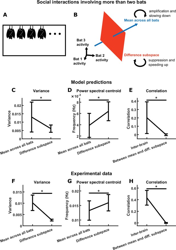
Group inter-brain relationship: model predictions and experimental tests.
(A) The two-bat model can be generalized to model the neural activity of a group of more than two socially interacting bats (the -bat model). (B) The mechanism underlying the -bat model, illustrated for the case of bats (three was chosen here only because higher-dimensional spaces cannot be illustrated). Shown are the mean component and the difference subspace in the activity space of bats. The mean component, corresponding to the mean activity across all bats, is a vector pointing towards the first octant. The difference subspace is the -dimensional subspace orthogonal to the direction of the mean component, and it contains all inter-brain activity patterns that correspond to activity differences across brains. Similar to the two-bat model, functional across-brain coupling acts as positive feedback to the -bat mean component, amplifying it and slowing it down; and as negative feedback to activity patterns in the difference subspace, suppressing them and speeding them up. (C)-(E) Model predictions from simulations of an -bat model where . Plotted are averages (± standard deviation) across simulations. (C) Model predictions on the variance of the mean component and the average variance of the difference subspace (total variance in the difference subspace divided by ). (D) Model predictions on the power spectral centroid of the mean component and the average power spectral centroid of the difference subspace (averaged across the power spectral centroids of activity in 1000 random directions in the difference subspace for a given simulation). (E) The model predicts positive inter-brain correlation and zero average correlation between the mean component and activity patterns in the difference subspace. Here, for each simulation, inter-brain correlation was averaged across all pairs of bats, and average correlation was calculated between the mean component and activity in 1000 random directions in the difference subspace. (F)-(H) Experimental tests. Neural activity was simultaneously recorded from the frontal cortices of four bats while they interacted in a chamber, under the same condition as the one-chamber sessions from Figure 1A. Mean normalized 30–150 Hz LFP power from the four bats were analyzed using the same methods as in (C)-(E). Note that the experimental results confirm the qualitative trends from the model predictions (although the data differ quantitatively from the predictions; see Materials and methods). *, p < 0.05, Wilcoxon signed rank test.


