Assessing target engagement using proteome-wide solvent shift assays
- Department of Cell Biology, Harvard Medical School, United States
Figures
Figure 1 with 3 supplements
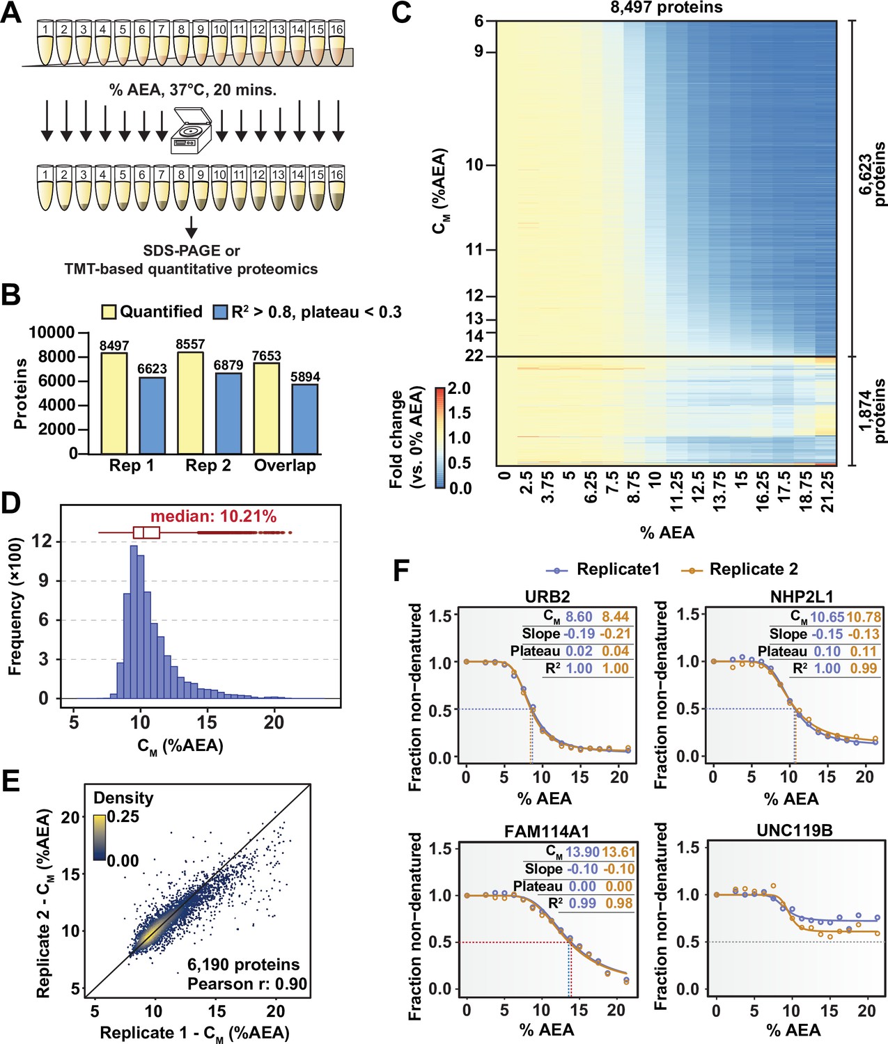
Solvent profiling of the HCT116 proteome.
(A) Schematic diagram of solvent-induced precipitation. (B) Count of quantified proteins in each replicate and those to which sigmoidal curves were fit well (R2 > 0.8 and plateau < 0.3). Each replicate is a single TMTpro 16plex experiment. (C) Heatmap representation of all proteins quantified in replicate 1. For each protein, its relative abundance (fold change) at the indicated %AEA compared to 0% AEA is presented. The proteins for which high-quality curves (R2 > 0.8 and plateau < 0.3) could be obtained (6623) are separated from those for which curves with reduced quality fits were returned (1874). Proteins are sorted by CM. (D) CM distribution for replicate 1. Proteins to which sigmoidal curves were fit well were included (6623 proteins, R2 > 0.8 and plateau < 0.3). (E) Reproducibility of CM measures between replicates. A high correlation (Pearson correlation – 0.9) was achieved. Proteins that showed high-quality curves (R2 > 0.8 and plateau < 0.3) in at least one replicate were included. (F) Examples of solvent melting curves for URB2, NHP2L1, FAM114A1, and UNC119B from replicate 1 (blue) and replicate 2 (orange). Inset in each panel reports CM, slope, plateau, and R2 for each curve. Curves were selected to highlight a range of CM values.
-
Figure 1—source data 1
Protein quantifications in the solvent-induced precipitation assay with 16 AEA concentrations (N = 2).
- https://cdn.elifesciences.org/articles/70784/elife-70784-fig1-data1-v1.xlsx
Figure 1—figure supplement 1
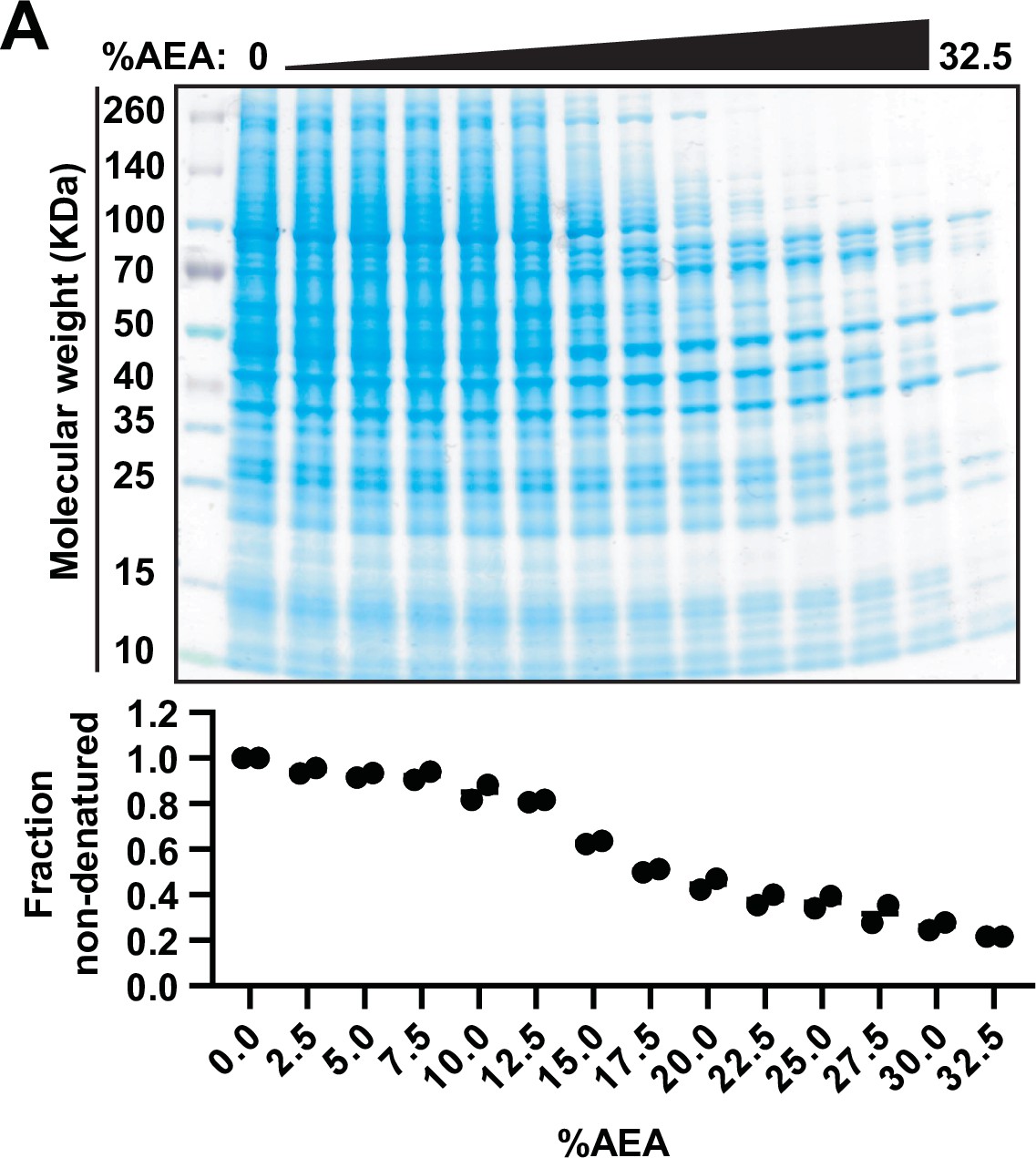
Solvent-induced denaturation of the HCT116 proteome.
Upper panel: native HCT116 lysates were treated with 14 increasing concentrations of AEA (0, 2.5, 5, 7.5, 10, 12.5, 15, 17.5, 20, 22.5, 25, 27.5, 30, 32.5%). Soluble fractions were resolved by SDS-PAGE and visualized with Coomassie staining.
Lower panel: the concentration of protein in each soluble fraction at each %AEA was determined by BCA assay from two biological replicates.
Figure 1—figure supplement 2
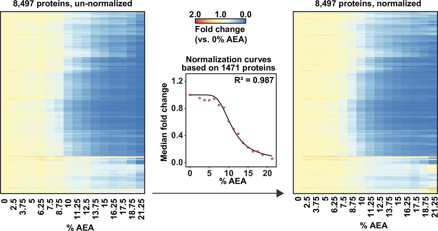
Solvent profiling of the HCT116 proteome.
Heatmap representation of all proteins quantified in replicate 1 before (left panel) and after (right panel) normalization with thermal proteome profiling (TPP) package. For each protein, its relative abundance (fold change) at the indicated %AEA compared to 0% AEA is presented.
Figure 1—figure supplement 3
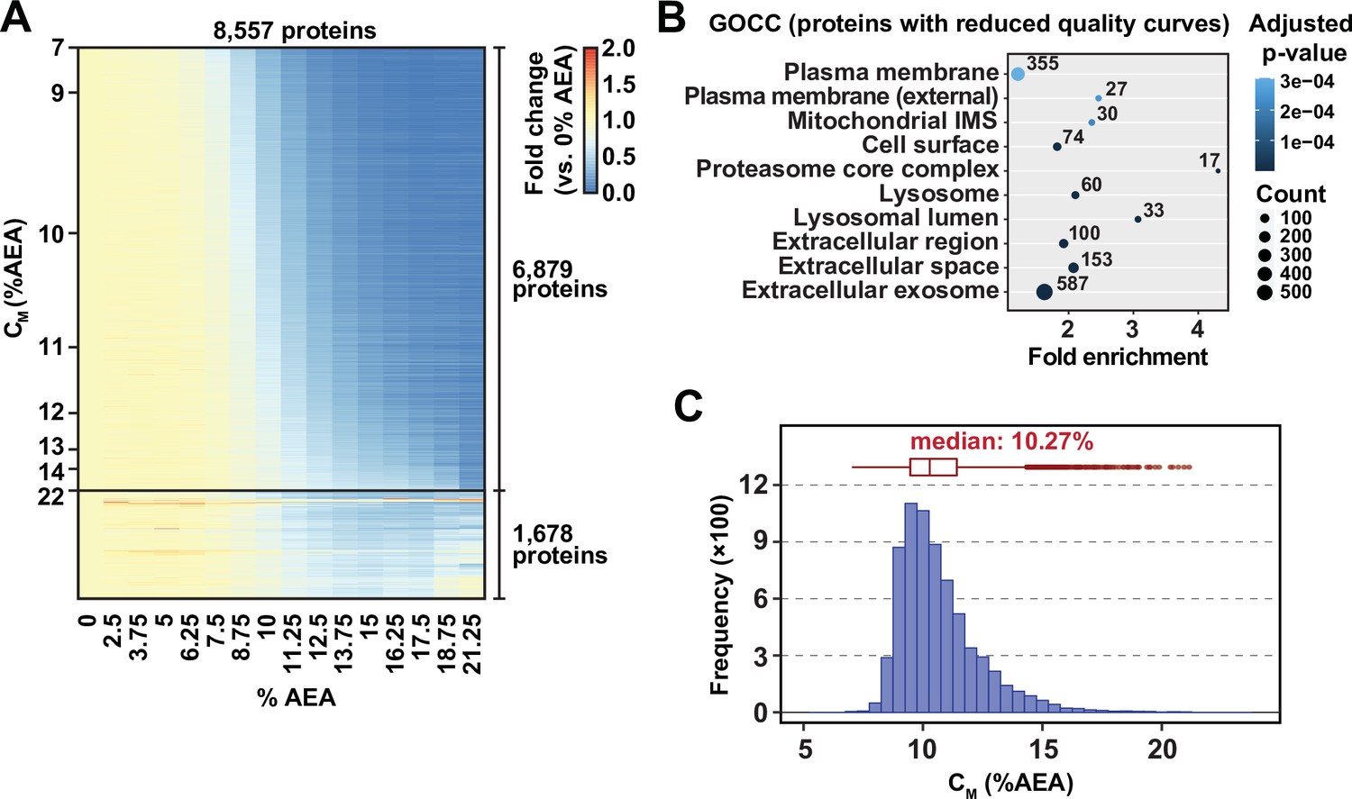
Solvent profiling of the HCT116 proteome.
(A) Heatmap representation of all proteins quantified in replicate 2. For each protein, its relative abundance (fold change) at the indicated %AEA compared to 0% AEA is presented. The proteins to which curves could be fit well (6879 proteins, R2 > 0.8 and plateau < 0.3) are separated from those to which curves could not be fit well (1678). Proteins are sorted by CM. (B) Gene Ontology enrichment analysis of proteins to which sigmoidal curves could not be fit well in replicate 1. (C) CM distribution in replicate 2. Proteins to which sigmoidal curves could be fit well are included (6879 proteins, R2 > 0.8 and plateau < 0.3).
Figure 2 with 3 supplements
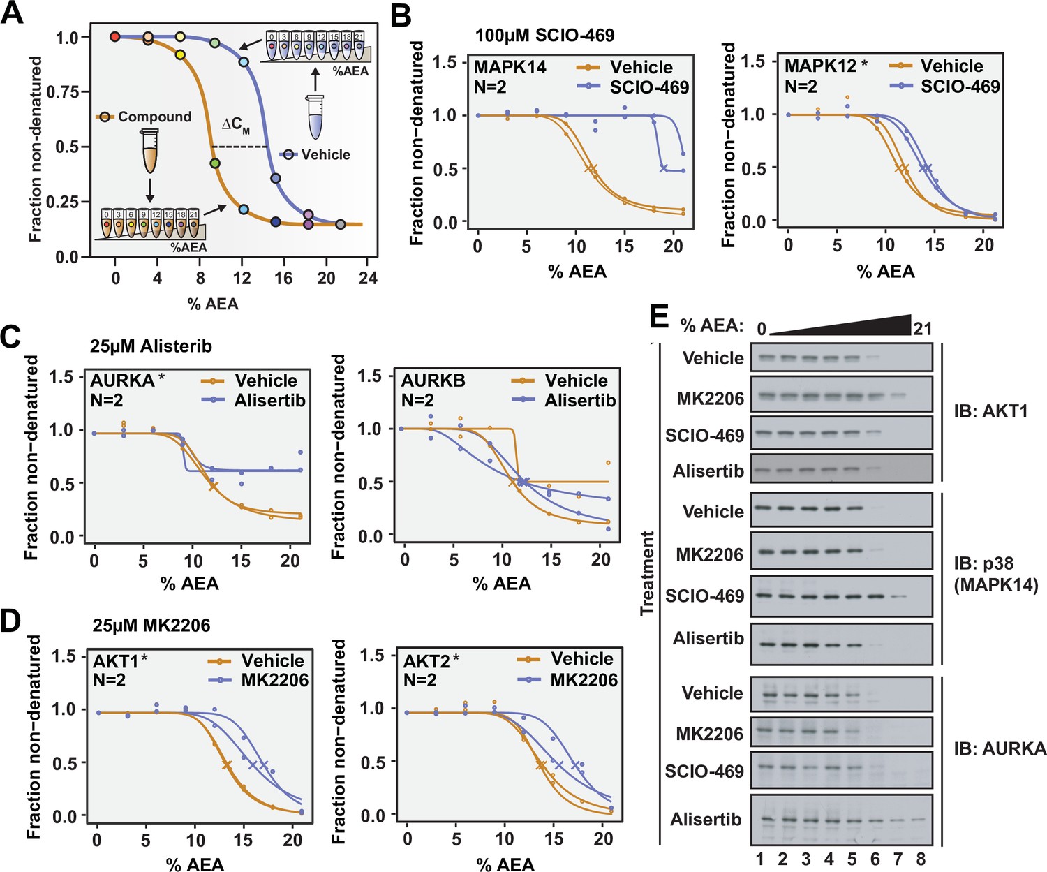
Solvent proteome profiling (SPP) can be used to determine compound target engagement.
(A) Schematic diagram summarizing the SPP workflow. (B) Native HCT116 lysates were treated with 100 μM SCIO-469. SPP melting curves for MAPK14 and MAPK12—known target proteins of SCIO-469—are displayed from two biological replicates. (C) Native HCT116 lysates were treated with 25 μM Alisertib. SPP melting curves for AURKA and AURKB are displayed for two biological replicates. (D) Native HCT116 lysates were treated with 25 μM MK2206. SPP melting curves for AKT1 and AKT2 are displayed for two biological replicates. (E) Soluble fractions from SPP were separated by SDS-PAGE and immunoblotted with the indicated antibodies. Asterisks indicate statistically significant hits (see Materials and methods). Crosses indicate melting points when available.
-
Figure 2—source data 1
Solvent proteome profiling (SPP) protein quantifications following treatment of HCT116 lysates with 100 µM SCIO-469 or vehicle.
N = 2.
- https://cdn.elifesciences.org/articles/70784/elife-70784-fig2-data1-v1.xlsx
-
Figure 2—source data 2
Solvent proteome profiling (SPP) protein quantifications following treatment of HCT116 lysates with 25 µM Alisertib or vehicle.
N = 2.
- https://cdn.elifesciences.org/articles/70784/elife-70784-fig2-data2-v1.xlsx
-
Figure 2—source data 3
Solvent proteome profiling (SPP) protein quantifications following treatment of HCT116 lysates with 25 µM MK-2206 or vehicle.
N = 2.
- https://cdn.elifesciences.org/articles/70784/elife-70784-fig2-data3-v1.xlsx
Figure 2—figure supplement 1
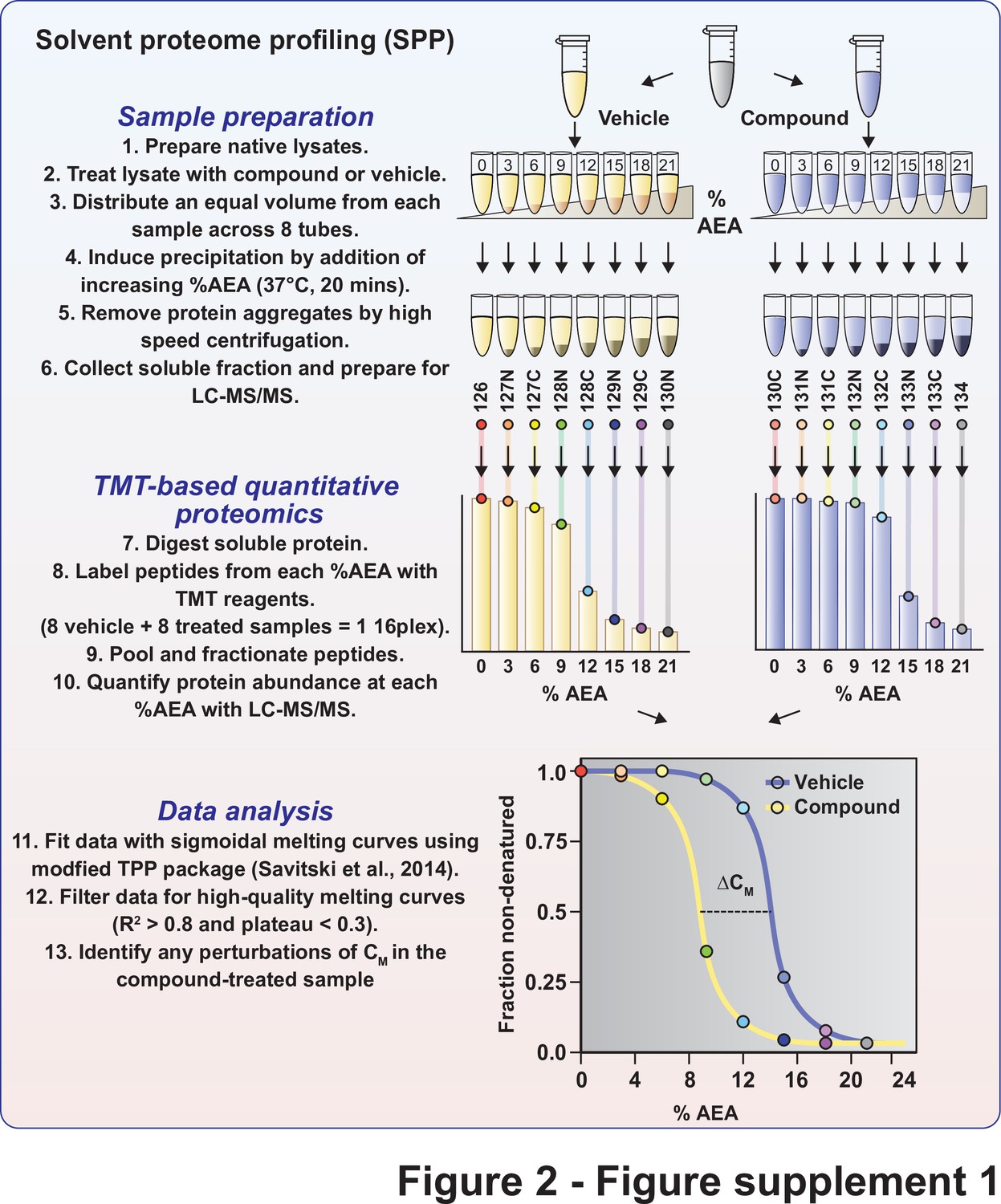
Schematic diagram of solvent proteome profiling (SPP).
Native cell lysates are prepared and divided into two aliquots. One aliquot is treated with drug and the other reserved for a vehicle-treated control. Samples are incubated with drug or vehicle for 15 min at room temperature. Compound- and vehicle-treated samples are further divided into eight aliquots and treated with increasing concentrations of AEA (0–3−6–9−12–15−18–21%). AEA-treated samples are incubated at 37°C for 20 min at which point they are subjected to centrifugation to separate the soluble and insoluble fractions. Soluble fractions are collected and the proteomes are reduced, alkylated, and digested. The resulting peptides were labeled with TMTpro 16plex reagents, pooled, and fractionated before being analyzed by LC-MS/MS. Sigmoidal protein denaturation curves were fit to the quantitative protein data. Target engagement is determined by a change in melting concentration (CM).
Figure 2—figure supplement 2
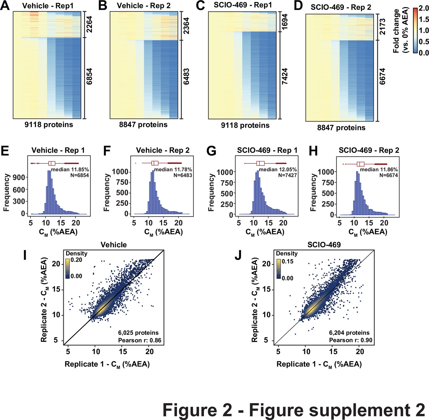
Solvent proteome profiling (SPP) of the HCT116 proteome.
(A–D) Heatmap representation of all proteins quantified in each replicate in the solvent proteome profiling (SPP) experiment with SCIO-469 treatment. For each protein, its relative abundance (fold change) at the indicated %AEA compared to 0% AEA is presented. The proteins to which curves could be fit well (R2 > 0.8 and plateau < 0.3) are separated from those for which curves with reduced quality fits. (E, F) The CM distribution for each replicate native HCT116 lysates treated with DMSO or SCIO-469. Only proteins showing high-quality curves were included (R2 > 0.8 and plateau < 0.3). (I, J) Reproducibility of CM measures between replicates treated with DMSO (I, Pearson correlation – 0.86) or SCIO-469 (J, Pearson correlation – 0.9). Proteins that showed high-quality curves (R2 > 0.8 and plateau < 0.3) in at least one replicate were included.
Figure 2—figure supplement 3
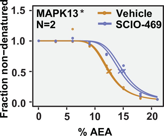
Solvent proteome profiling (SPP) can be used to determine compound target engagement.
Native HCT116 lysates were treated with 100 μM SCIO-469. Solvent melting curve for MAPK13 is displayed for two replicate experiments. Asterisks indicate statistically significant hits (see Materials and methods). Crosses indicate melting points when available.
Figure 3 with 3 supplements
Solvent-PISA can resolve compound target engagement with increased efficiency.
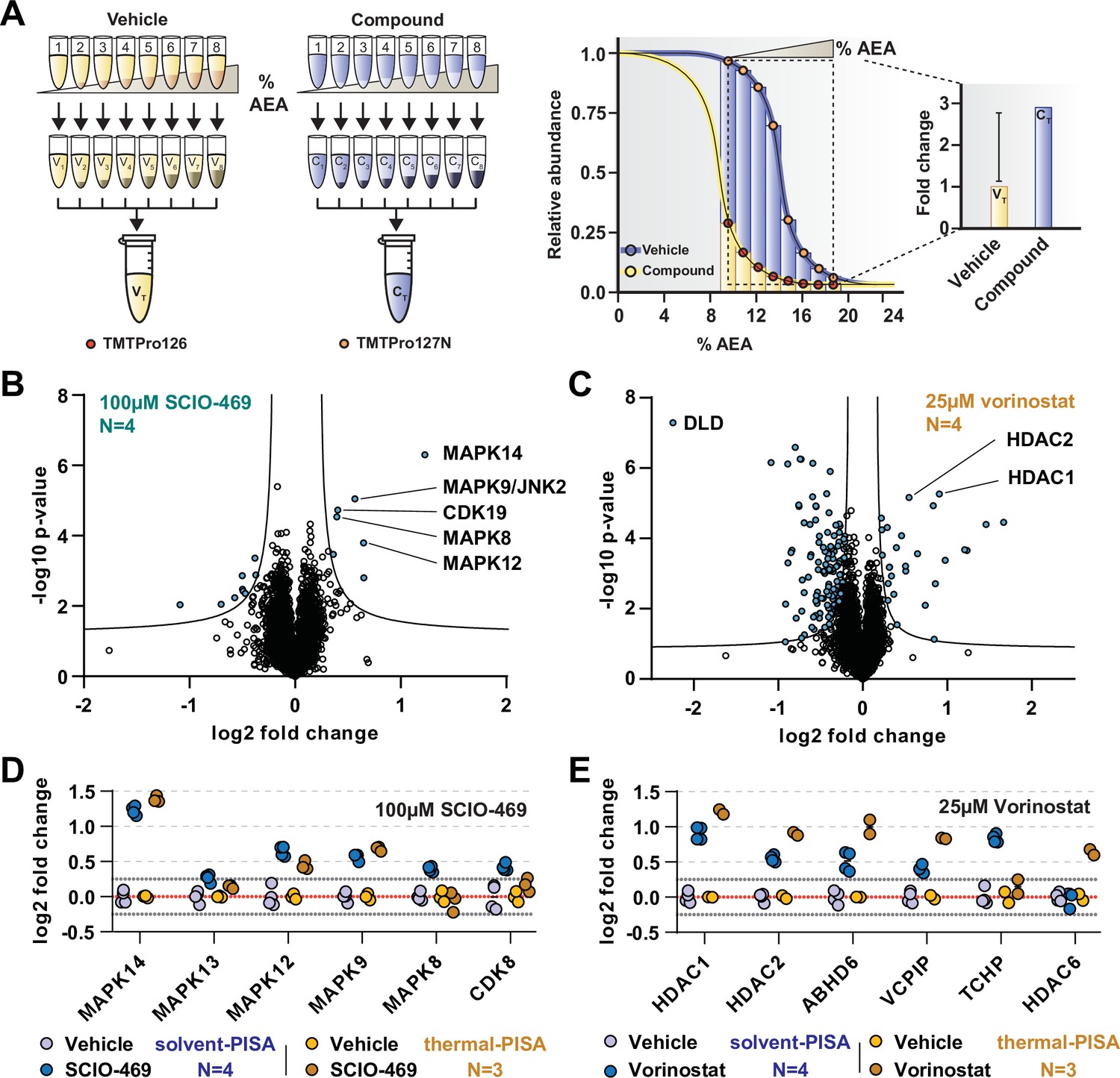
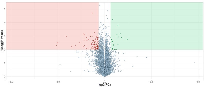
(A) Native cell lysates are prepared and divided into multiple aliquots. Half the aliquots are treated with drug and the other half reserved for a vehicle-treated control. Samples are incubated for 15 min at room temperature. Compound- and vehicle-treated samples are further divided into eight aliquots and treated with increasing concentrations of AEA (9, 10.375, 11.75, 13.125, 14.5, 15.875, 17.25, and 18.625%). AEA-treated samples are incubated at 37°C for 20 min at which point they are subjected to centrifugation to separate the soluble and insoluble fractions. Soluble fractions are collected and pooled in equal volumes before being reduced, alkylated, and digested. The resulting peptides are labeled with TMTpro 16plex reagents, pooled, and fractionated before being analyzed by LC-MS/MS. Target engagement is determined by an increase or decrease in protein content compared to the vehicle-treated control. (B, C) HCT116 lysates were treated with 100 μM SCIO-469 (B) or 25 μM vorinostat (C) and analyzed by solvent-PISA. Data are presented as a volcano plot to highlight significant changes in abundance. Significant changes were determined using a permutation-based false discovery rate (FDR) (FDR – 0.05, S0 – 0.1) and are indicated with blue dots. (D, E) HCT116 lysates were treated with 100 μM SCIO-469 (D) or 25 μM vorinostat (E) and analyzed by solvent-PISA (blue shades) or thermal-PISA (orange shades). Individual log2 fold change values (in reference to the vehicle mean) are plotted for several proteins. Dotted lines at y = 0.25 and y = −0.25 are included to denote fold change values of ~20%.
-
Figure 3—source data 1
Solvent-PISA and thermal-PISA protein quantifications following treatment of HCT116 lysates with 100 µM SCIO-469 or vehicle (N = 4).
- https://cdn.elifesciences.org/articles/70784/elife-70784-fig3-data1-v1.xlsx
-
Figure 3—source data 2
Solvent-PISA and thermal-PISA protein quantifications following treatment of HCT116 lysates with 25 µM vorinostat or vehicle (N = 4).
- https://cdn.elifesciences.org/articles/70784/elife-70784-fig3-data2-v1.xlsx
Figure 3—figure supplement 1
Solvent-PISA can resolve compound target engagement with increased efficiency.
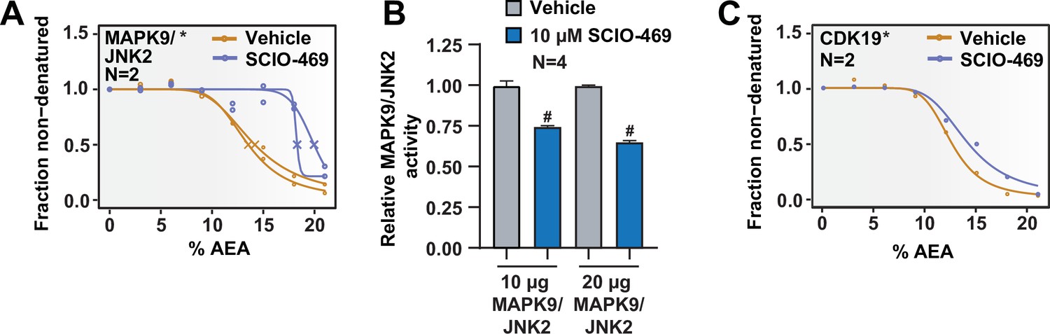
(A) Solvent melting curves for MAPK9. (B) MAPK9/JNK2 in vitro kinase assay. Bars represent the mean relative kinase activity of four replicate measurements with (blue) and without (gray) 10 µM SCIO-469. Data represent two independent experiments in which 10 µg or 20 µg MAPK9/JNK2 was used per reaction. #p<0.0001. (C) Solvent melting curves for MAPK9/JNK2. Asterisks indicate statistically significant hits (see Materials and methods). Crosses indicate melting points when available.
Figure 3—figure supplement 2
Solvent-PISA can resolve compound target engagement with increased efficiency.
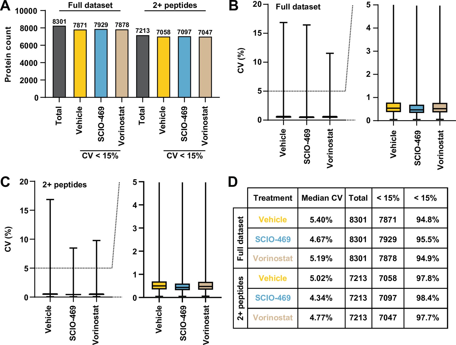
(A) Count of total proteins quantified and proteins quantified with at least two peptides and with a %CV < 15% across replicates. (B, C) Distribution of CV values from each experimental group for all proteins quantified (B) and those quantified with at least two peptides (C). For the box plots, center line, median; box limits correspond to the first and third quartiles; whiskers, 1.5× interquartile range, outliers not shown. (D) Table summarizing the filters used during data analysis. A significant change in CM is defined by p<0.0001.
Figure 3—figure supplement 3
Solvent-PISA can resolve compound target engagement with increased efficiency.
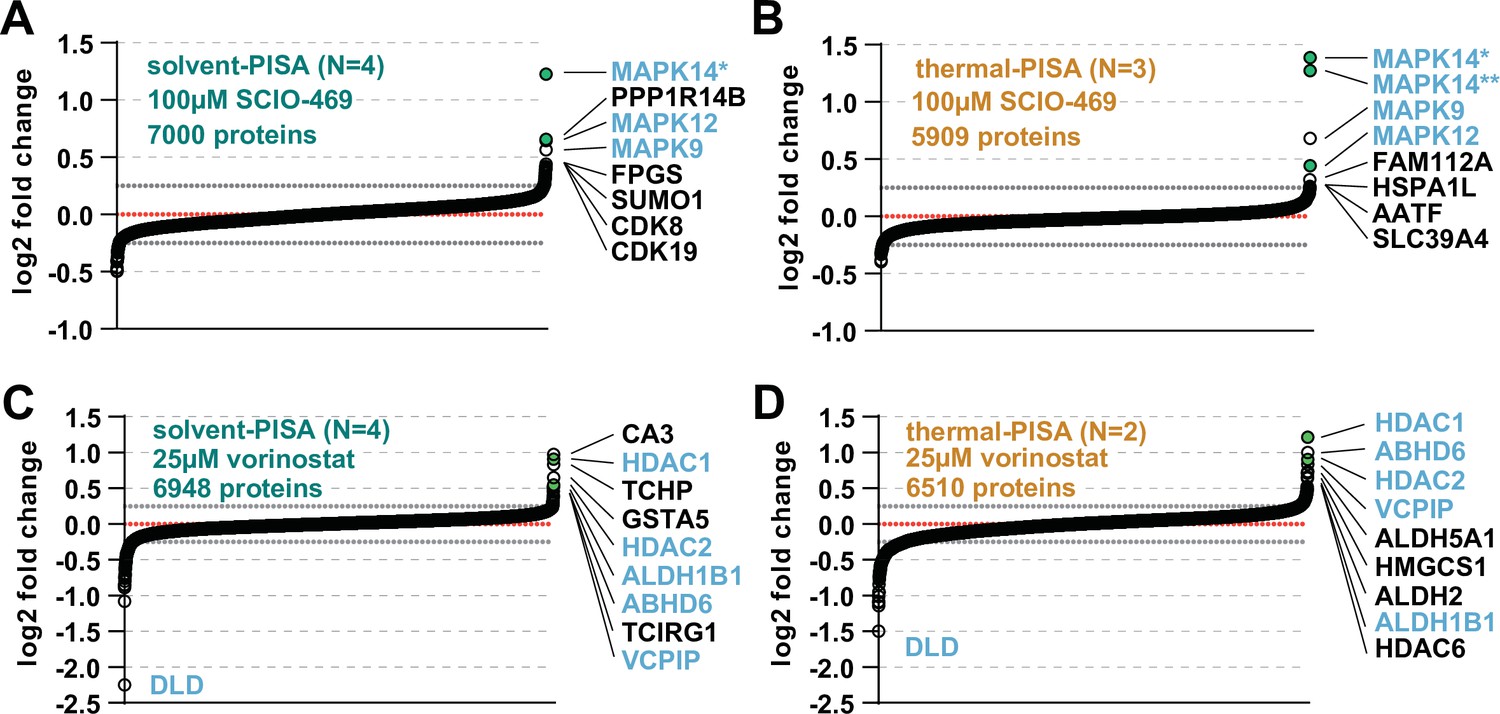
(A, B) HCT116 lysates were treated with 100 μM SCIO-469 and analyzed by solvent-PISA (A) or thermal-PISA (B). Proteins quantified with at least two peptides and having a %CV < 15 across replicates were sorted by the mean log2 fold change of four (A) or three (B) replicate measurements. (C, D) HCT116 lysates were treated with 25 μM vorinostat and analyzed by solvent-PISA (C) or thermal-PISA (D). Proteins quantified with at least two peptides and having a %CV < 15% across replicates were sorted by the mean log2 fold change of four (C) or two (D) replicate measurements. Known targets are indicated with green dots. Dotted lines at y = 0.25 and y = −0.25 are included to highlight significant shifts. * indicate different isoforms of the same gene.
Figure 4 with 2 supplements
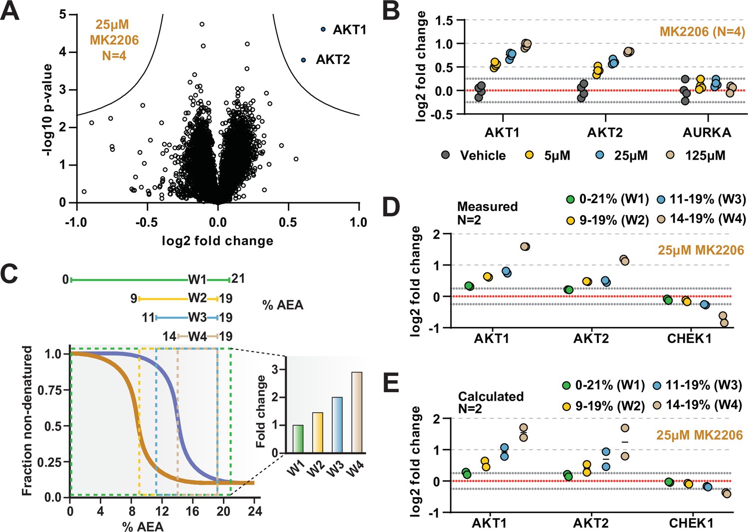
The range of AEA concentrations used in a solvent-PISA experiment impacts the ultimate fold change measurements.
(A) HCT116 lysates were treated with 25 μM MK2206 and analyzed by solvent-PISA. Data are presented as a volcano plot to highlight significant changes in abundance. Significant changes were determined using a permutation-based false discovery rate (FDR) (FDR – 0.05, S0 – 0.1) and are indicated with blue dots. (B) HCT116 lysates were treated with 5 μM, 25 μM, or 125 μM MK2206 and analyzed by solvent-PISA. Individual log2 fold change values are plotted for several proteins at each concentration. Dotted lines at y = 0.25 and y = −0.25 are included to highlight minimum changes of ~20%. (C) Schematic diagram of solvent proteome profiling (SPP) melting curves indicating the range of %AEA used for each window. (D) Individual log2 fold change values are plotted for several proteins measured using different windows. (E) Expected log2 fold change values for several proteins were calculated based on SPP melting curves determined by SPP for each window (calculated from Figure 2B). Individual abundances for the compound-treated samples and vehicle-treated controls at each %AEA within a given range were summed. Considering the 0–21% window (window 1), for example, we simply summed all eight abundance measurements from the eight AEA concentrations used to generate the SPP data. For the 9–19% window (window 2), we summed only the SPP abundances between 9 and 19%, and so on.
-
Figure 4—source data 1
Solvent-PISA protein quantifications following treatment of HCT116 lysates with 25 µM Alisertib or vehicle (N = 4).
- https://cdn.elifesciences.org/articles/70784/elife-70784-fig4-data1-v1.xlsx
-
Figure 4—source data 2
Solvent-PISA protein quantifications following treatment of HCT116 lysates with 25 µM MK2206 or vehicle (N = 4).
- https://cdn.elifesciences.org/articles/70784/elife-70784-fig4-data2-v1.xlsx
-
Figure 4—source data 3
Solvent-PISA protein quantifications following treatment of HCT116 lysates with 25 µM MK2206 or vehicle across four solvent-PISA windows (see Materials and methods) (N = 2).
- https://cdn.elifesciences.org/articles/70784/elife-70784-fig4-data3-v1.xlsx
Figure 4—figure supplement 1
The range of AEA concentrations used in a solvent-PISA experiment impacts the ultimate fold change measurements.
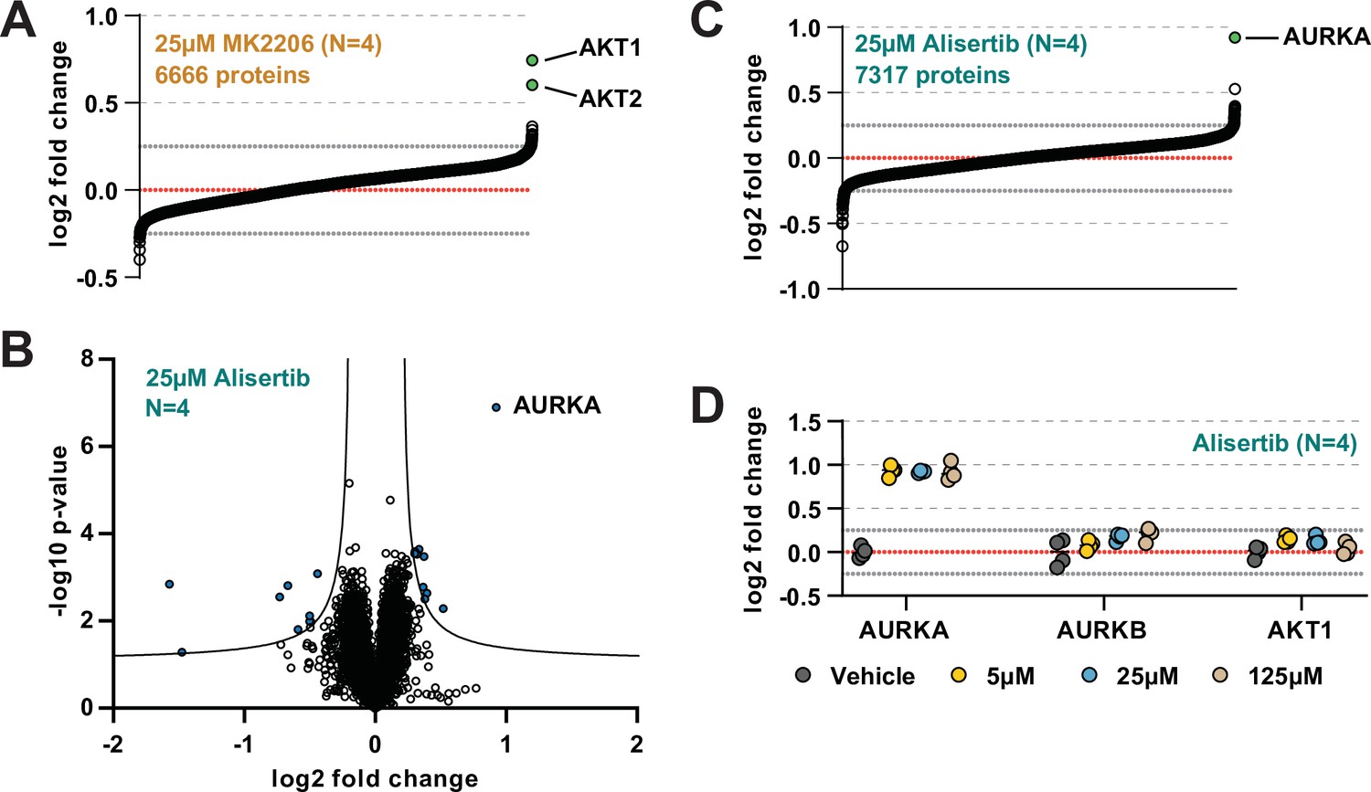
(A) HCT116 lysates were treated with 25 μM MK2206 and analyzed by solvent-PISA. Proteins quantified with at least two peptides and having a %CV < 15 across replicates were sorted by the mean log2 fold change of four replicate measurements. (B) HCT116 lysates were treated with 25 μM Alisertib and analyzed by solvent-PISA. Data are presented as a volcano plot to highlight significant changes in abundance. Significant changes were determined using a permutation-based false discovery rate (FDR) (FDR – 0.05, S0 – 0.1) and are indicated with blue dots. (C) HCT116 lysates were treated with 25 μM Alisertib and analyzed by solvent-PISA. Proteins quantified with at least two peptides and having a %CV < 15 across replicates were sorted by the mean log2 fold change of four replicate measurements. (D) Individual log2 fold change values are plotted for several proteins at each concentration of Alisertib. Dotted lines at y = 0.25 and y = −0.25 are included to highlight changes of ~20%.
Figure 4—figure supplement 2
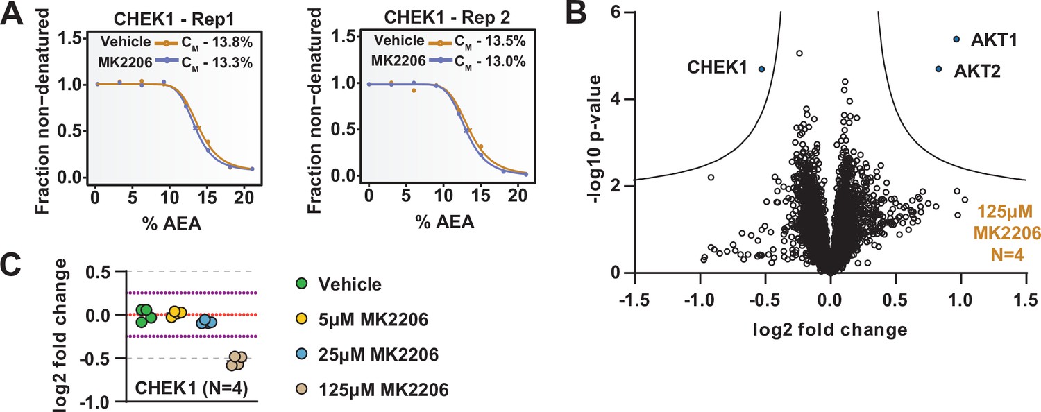
The range of AEA concentrations used in a solvent-PISA experiment impacts the ultimate fold change measurements.
(A) Solvent proteome profiling (SPP) melting curves for CHEK1. Replicate experiments were separated into two different panels for visualization. (B) HCT116 lysates were treated with 125 μM MK2206 and analyzed by solvent-PISA. Data are presented as a volcano plot to highlight significant changes in abundance. Significant changes were determined using a permutation-based false discovery rate (FDR) (FDR – 0.05, S0 – 0.1) and are indicated with blue dots. (C) HCT116 lysates were treated with 5 μM, 25 μM, or 125 μM MK2206 and analyzed by solvent-PISA. Individual log2 fold change values for CHEK1 are displayed at each concentration of MK2206. All values are derived from a single TMTpro 16plex experiment.
Figure 5 with 1 supplement
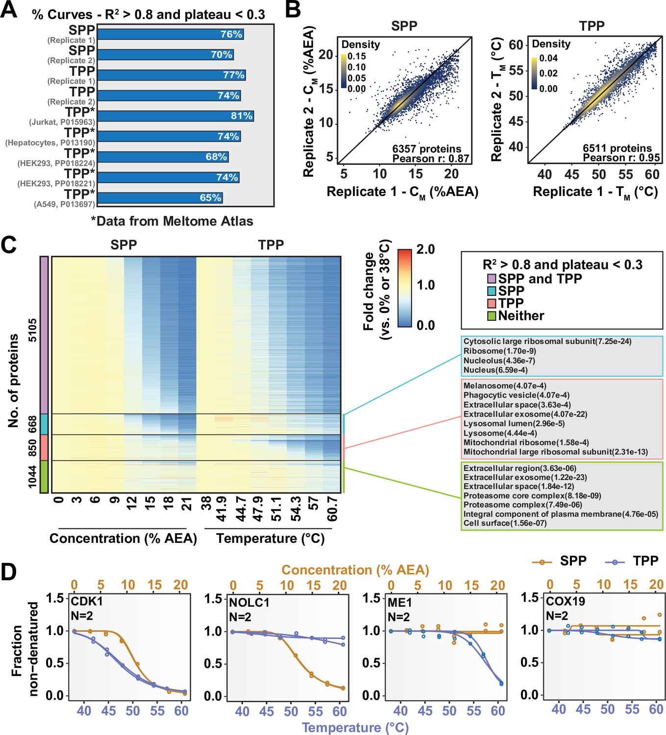
Combining solvent proteome profiling (SPP) with thermal proteome profiling (TPP) to maximize proteome coverage.
(A) Fractions of high-quality curves (R2 > 0.8 and plateau < 0.3) in SPP and TPP datasets. * indicates datasets taken from the Meltome Atlas (Jarzab et al., 2020). A similar fraction (~70%) of high-quality curves were obtained in SPP and TPP assays. (B) Reproducibility of SPP CM (left panel) and TPP TM (right panel) values between replicates. SPP and TPP experiments showed equivalent reproducibility between replicates. Proteins that show high-quality curves (R2 > 0.8 and plateau < 0.3) in at least one replicate were included. (C) Heatmap representation of all proteins quantified in both SPP and TPP (replicate 1). For each protein, its relative abundance (fold change) at the indicated %AEA compared to 0% AEA (SPP, left) or at the indicated temperature compared to 38°C (TPP, right) is presented. The panel on the right indicates Gene Ontology entries that are enriched in each indicated group. Proteins that were quantified in both SPP and TPP were used as the background. (D) Selected SPP (orange) and TPP (blue) denaturation/melting curves highlighting proteins showing high-quality curves (R2 > 0.8 and plateau < 0.3) in both approaches, in SPP alone (second), in TPP alone (third), or neither (fourth).
-
Figure 5—source data 1
Solvent proteome profiling (SPP) and thermal proteome profiling (TPP) protein quantifications (eight AEA concentrations or eight temperatures) (N = 2).
- https://cdn.elifesciences.org/articles/70784/elife-70784-fig5-data1-v1.xlsx
Figure 5—figure supplement 1
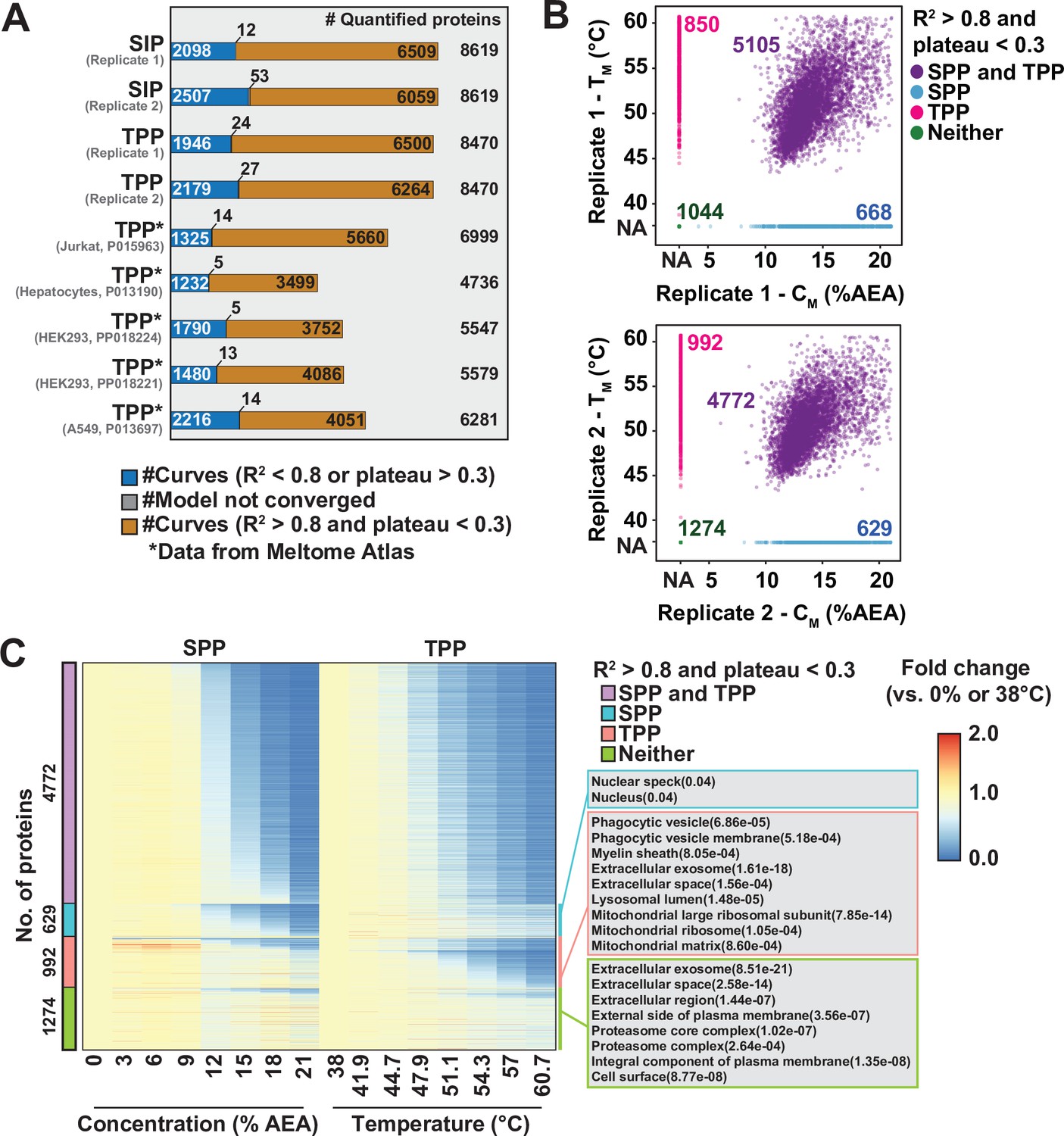
Combining SPP with TPP to maximize proteome coverage.
(A) Total number of high-quality curves (R2 > 0.8 and plateau < 0.3) in solvent proteome profiling (SPP) and thermal proteome profiling (TPP) datasets. * indicates datasets taken from the Meltome Atlas (Jarzab et al., 2020). (B) Relationship between CM (x-axes) and TM (y-axes) for two replicate experiments. (C) Heatmap representation of all proteins quantified in both SPP and TPP (replicate 2). For each protein, its relative abundance (fold change) at the indicated %AEA compared to 0% AEA (SPP, left) or at the indicated temperature compared to 38°C (TPP, right) is presented. The panel on the right indicates Gene Ontology entries that are enriched in each indicated group. Proteins quantified in both SPP and TPP were used as the background. For proteins (colored in cyan) showing good curves in SPP, but not in TPP, adjusted p-values were filtered at 0.05.
Author response image 1
HCT116 lysates were treated with 25 µM vorinostat and assays by thermal-PISA (N=2).
We included this explanation in the Results section of the main text (page 10).
Tables
Key resources table
| Reagent type (species) or resource | Designation | Source or reference | Identifiers | Additional information |
|---|---|---|---|---|
| Cell line (Homo sapiens) | HCT116 (adult, colorectal cancer) | ATCC | Cat# CCL-247 | Male |
| Antibody | Anti-Akt (rabbit monoclonal) | Cell Signaling Technology | Cat# 4691 | WB (1:1000) |
| Antibody | Anti-p38 MAPK (rabbit polyclonal) | Cell Signaling Technology | Cat# 9212 | WB (1:1000) |
| Antibody | Anti-Aurora A (rabbit monoclonal) | Cell Signaling Technology | Cat# 4718 | WB (1:1000) |
| Antibody | Goat anti-rabbit IgG-HRP | Santa Cruz | Cat# sc-2004 | WB (1:10,000) |
| Chemical compound, drug | SCIO-469 | Cayman Chemical | Cat# 29484;batch: 0575761-1 | 10 µM stock in DMSO |
| Chemical compound, drug | Alisertib(MLN8237) | Cayman Chemical | Cat# 13602;batch: 0565558-18 | 10 µM stock in DMSO |
| Chemical compound, drug | MK2206 (hydrochloride) | Cayman Chemical | Cat# 11593;batch: 0586491-5 | 10 µM stock in DMSO |
| Chemical compound, drug | Vorinostat(SAHA) | Cayman Chemical | Cat# 10009929;batch: 0512249-52 | 10 µM stock in DMSO |
| Commercial assay or kit | TMTpro 16plex Label Reagent Set | Thermo Fisher | Cat# A44520;batch: VI313212 | Solubilized in anhydrous acetonitrile |
| Commercial assay or kit | JNK2 kinase enzyme | Promega | Cat# VA7210 | |
| Commercial assay or kit | ADP-Glo kinase assay | Promega | Cat# V9101 | |
| Software, algorithm | Perseus | ttp://maxquant.net/perseusTyanova et al., 2016 | Version 1.6.15.0 | |
| Software, algorithm | Prism | GraphPad | Version 9.0.0 | |
| Software, algorithm | R | https://www.r-project.org/ | Version 4.0.2 | |
| Software, algorithm | TPP package | https://github.com/DoroChilds/TPP; Franken et al., 2015 | Version 3.17.6 | |
| Other | Sera-Mag SpeedBead Carboxylate-Modified Magnetic Particles (Hydrophobic) | Cytiva | Cat# 44152105050250 | |
| Other | Sera-Mag Carboxylate-Modified Magnetic Particles (Hydrophylic) | Cytiva | Cat#45152105050250 |
Additional files
Download links
A two-part list of links to download the article, or parts of the article, in various formats.
Downloads (link to download the article as PDF)
Open citations (links to open the citations from this article in various online reference manager services)
Cite this article (links to download the citations from this article in formats compatible with various reference manager tools)
Assessing target engagement using proteome-wide solvent shift assays
eLife 10:e70784.
https://doi.org/10.7554/eLife.70784


