Synaptic connectivity to L2/3 of primary visual cortex measured by two-photon optogenetic stimulation
- Allen Institute for Brain Science, United States
Figures
Figure 1 with 3 supplements
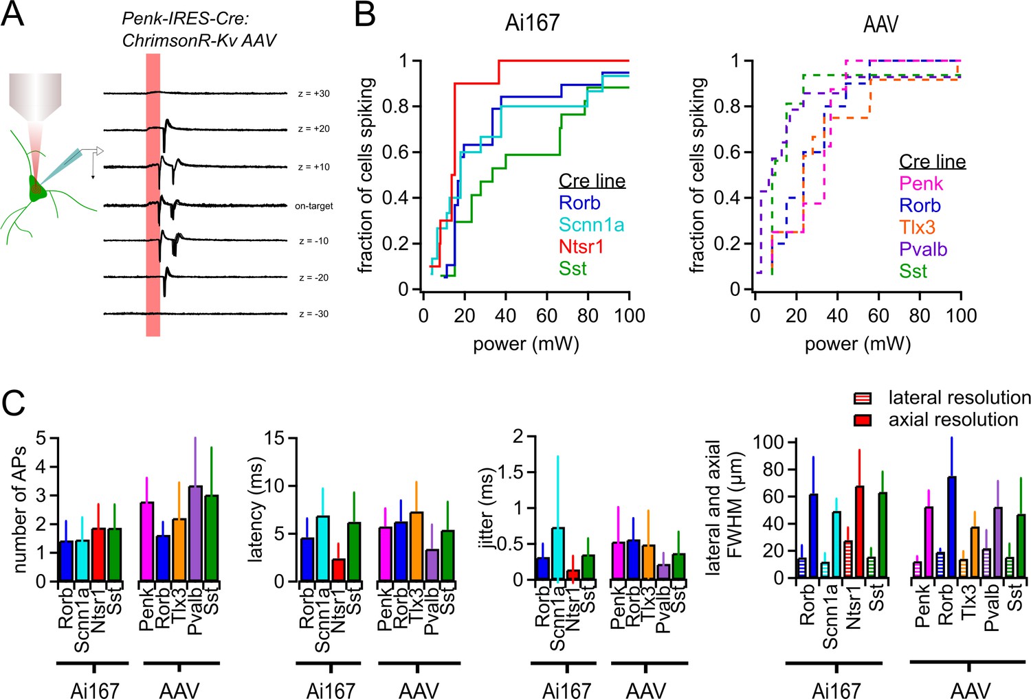
Characterization of two-photon-evoked spiking.
(A) Examples of action potentials (APs) evoked by two-photon stimulation of a Penk-Cre neuron with indicated axial offsets. Each offset includes 10 overlaid sweeps. Stimulus duration was 10 ms (red shaded bar). (B) Cumulative probability of light-evoked spiking versus photostimulus power for the indicated Cre lines crossed to Ai167 or injected with AAV carrying soma-targeted ChrimsonR. (C) The average number of APs evoked per photostimulus, latency, jitter, and spatial resolution of photostimulation (measured using the same power used for mapping experiments) for all Cre line and opsin expression strategies used in this study. Error bars represent standard deviation across cells. Minimum power, latency, and jitter data were collected from a total of 123 neurons (8–19 neurons per Cre line-expression method combination). Lateral resolution was measured from a total of 66 neurons (5–12 per Cre line-expression method combination. Axial resolution was measured from a total of 78 neurons (6–13 per Cre line-expression method combination)).
-
Figure 1—source data 1
Raw values for plots in Figure 1.
- https://cdn.elifesciences.org/articles/71103/elife-71103-fig1-data1-v2.xlsx
Figure 1—figure supplement 1
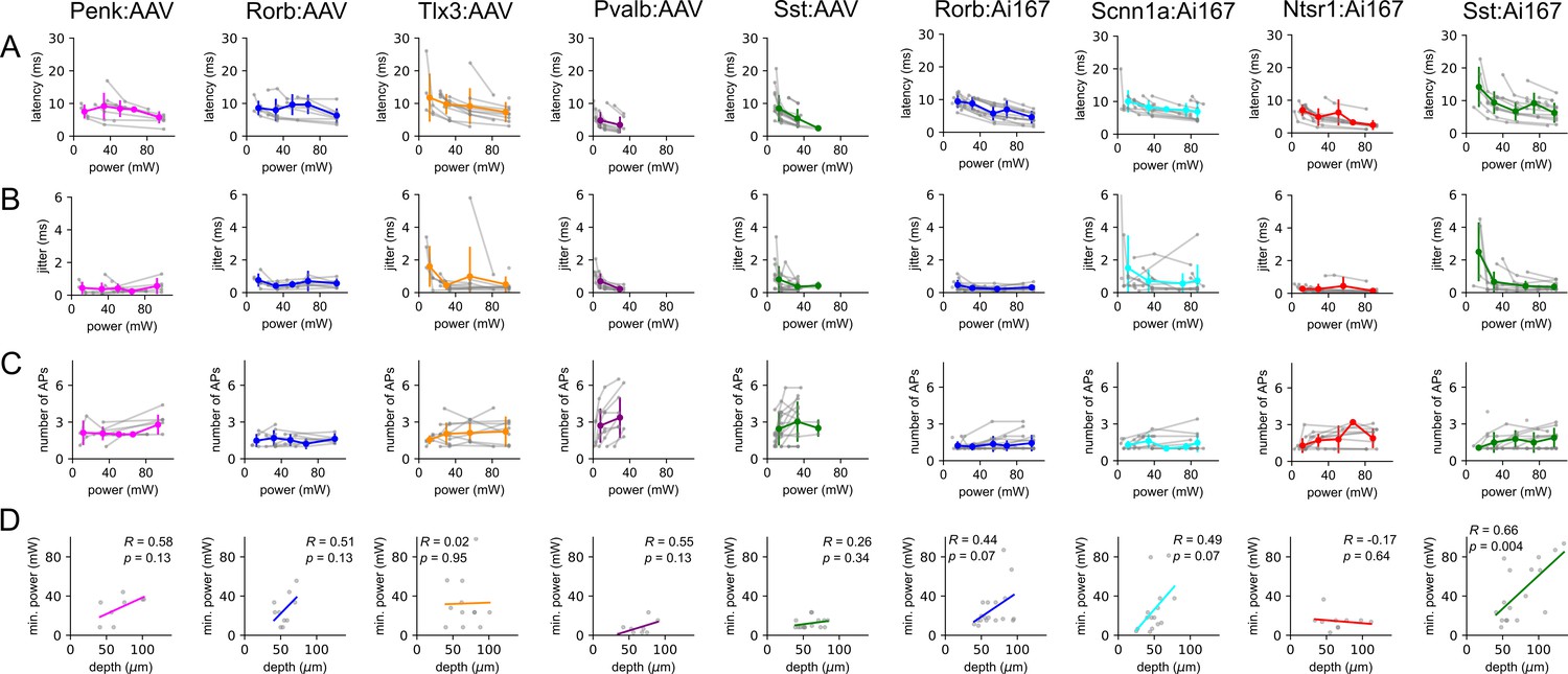
Characterization of spiking evoked by two-photon stimulation.
Columns represent data collected from the indicated Cre line crossed to the Ai167 effector line (ChrimsonR-tdTomato expressing) or injected with adeno-associated virus (AAV) carrying FLEX’ed soma-targeted-ChrimsonR (ChrimsonR-EYFP-Kv2.1). Each row represents the indicated measurement. Data are plotted for individual neurons (gray) with average values measured for each Cre line/effector combination (color) binned in 20 mW intervals. Error bars represent the standard deviation across cells. Data were collected from a total of 123 neurons (8–19 neurons per Cre line/effector combination). (A) Latency to first action potential (AP) versus photostimulus power. (B) Jitter of first AP versus photostimulus power. (C) Number of APs versus photostimulus power. (D) Minimum power required to evoked reliable spiking (on 10/10 trials) versus depth of the cell from the surface the slice. Colored lines represent linear fit to the data. Pearson’s R and associated p-values are presented as insets for each plot.
-
Figure 1—figure supplement 1—source data 1
Raw values for plots in Figure 1—figure supplement 1.
- https://cdn.elifesciences.org/articles/71103/elife-71103-fig1-figsupp1-data1-v2.xlsx
Figure 1—figure supplement 2
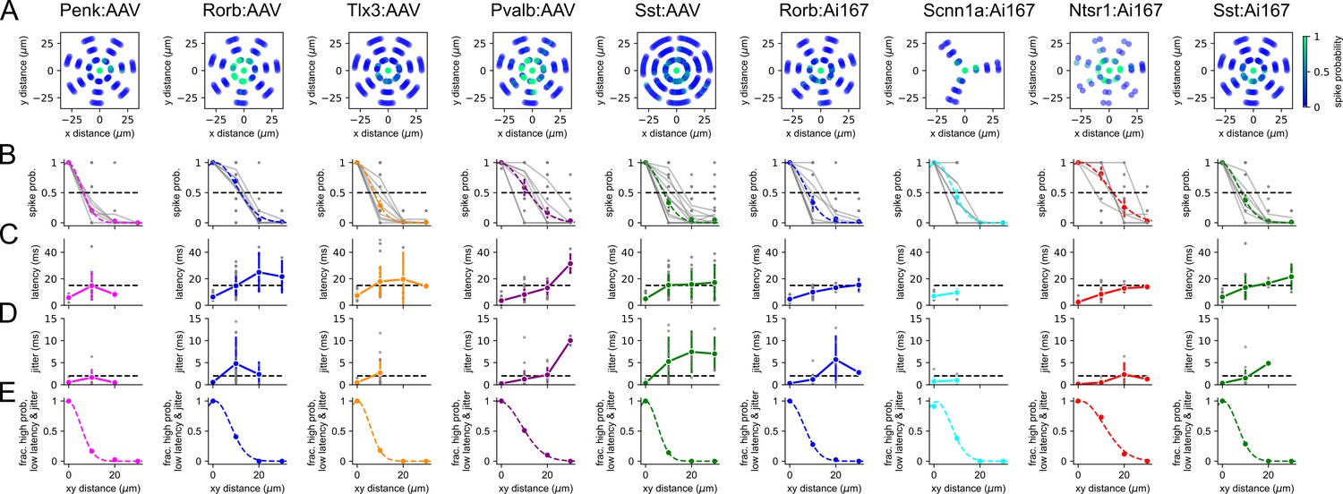
Lateral resolution of spiking evoked by two-photon stimulation.
Columns represent data collected from the indicated Cre line crossed to the Ai167 effector line (ChrimsonR-tdTomato expressing) or injected with adeno-associated virus (AAV) carrying FLEX’ed soma-targeted-ChrimsonR (ChrimsonR-EYFP-Kv2.1). Lateral resolution was measured from a total of 66 neurons (5–12 per Cre line/effector combination) using the same parameters as mapping experiments. (A) Heatmaps of action potential (AP) probability plotted against x and y distances of the photostimulus from the center of the cell. The target was offset in a wagon-wheel pattern at distances of 10, 20, and 30 µm from the center of the soma. For most experiments, lateral resolution was measured in seven different directions from the soma. Experiments with Scnn1a-Cre tested lateral resolution in fewer directions (three) but yielded similar estimates of lateral resolution. For display purposes, data from each experiment were iteratively rotated by 3 degrees to reduce overlap of data points. (B–D) Spike probability, latency to first AP, and jitter plotted against lateral (xy) distance from the center of the recorded cell. Data are plotted for individual measurements (gray) with average values measured for each Cre line/effector combination (color). In row (B), average values of spike probability versus distance were fit with a Gaussian function (dashed colored line). (E) The fraction of photostimulus locations that produced reliable (spike probability > 0.5), low-latency (<15 ms), high-precision (jitter < 2 ms) AP firing versus lateral distance from the soma. Criteria are represented as horizontal dashed lines in rows (B) – (D).
Figure 1—figure supplement 3
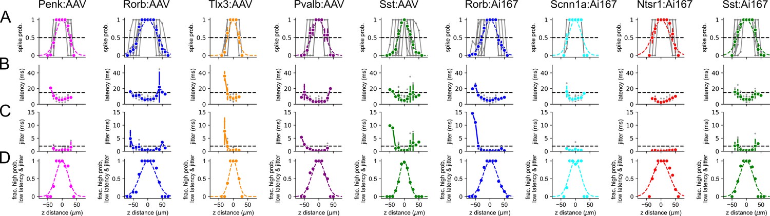
Axial resolution of spiking evoked by two-photon stimulation.
Columns represent data collected from the indicated Cre line crossed to the Ai167 effector line (ChrimsonR-tdTomato) or injected with adeno-associated virus (AAV) carrying FLEX’ed soma-targeted-ChrimsonR (ChrimsonR-EYFP-Kv2.1). Axial resolution was measured from a total of 78 neurons (6–13 per Cre line/effector combination) using the same parameters as mapping experiments. (A–C) Spike probability, latency to first action potential (AP), and jitter plotted against axial (z) distance from the center of the recorded cell. Data are plotted for individual measurements (gray) with average values measured for each Cre line/effector combination (color). In row (A), average values of spike probability versus distance were fit with a Gaussian function (dashed colored line). (D) The fraction of photostimulus locations that produced reliable (spike probability > 0.5), low-latency (<15 ms), low-jitter (<2 ms) AP firing versus lateral distance from the soma. Criteria are represented as horizontal dashed lines in rows (A) – (C).
Figure 2 with 1 supplement
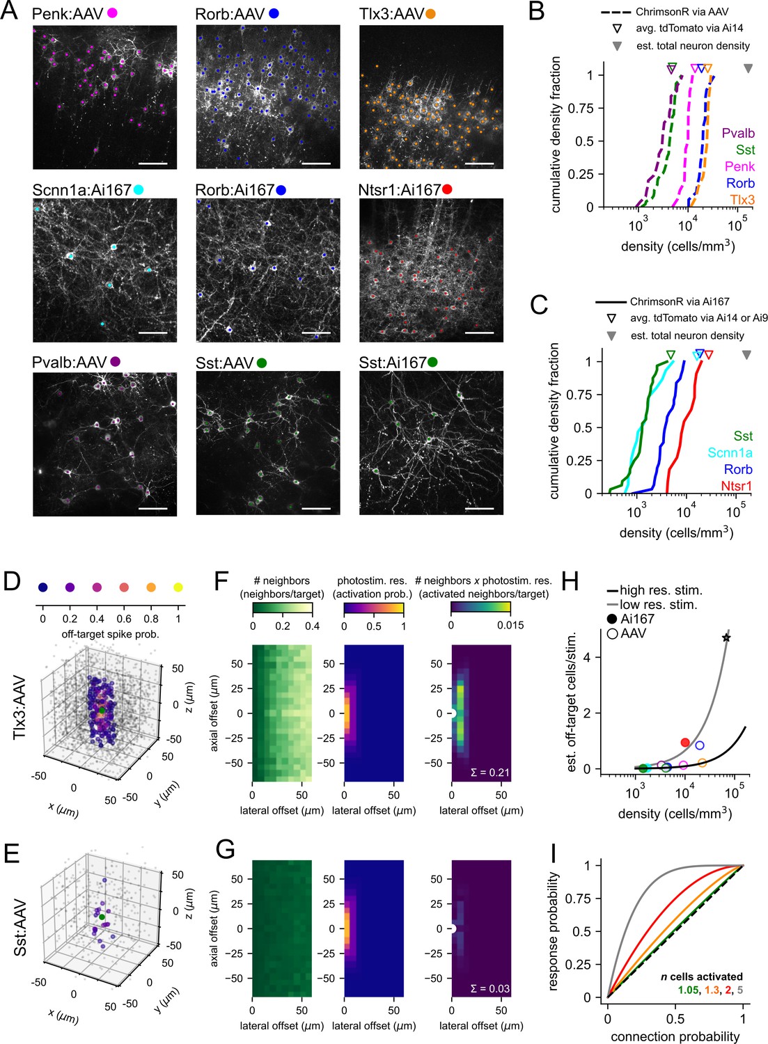
Labeled cell densities and estimates of off-target activation.
(A) Example images for all Cre lines and expression method combinations used in this study. Two-photon z-stacks were collected at the conclusion of mapping experiments. Each image shown is a maximum intensity projection of a 40 µm subset of the axial/z dimension. Scale bars = 60 µm. The positions of labeled cells were manually annotated in three dimensions (colored dots, z location not represented here). (B) Cumulative distributions of labeled cell densities measured across multiple experiments using adeno-associated virus (AAV) (dashed lines). Distributions are color-coded by Cre line as in panel (A). Open triangles represent the mean density of labeled cells measured from Ai14 adult mice crossed to the same Cre lines. Filled gray triangle represents the average reported total neuron density in mouse visual areas (Keller et al., 2018). (C) Same as panel (B) for experiments using Ai167-mediated ChrimsonR expression. (D) For 100 randomly selected neurons in the Tlx3:AAV dataset (overlaid green circles), the relative location of all identified neighboring cells s plotted and color-coded by estimated off-target activation probability (note warmer colors near the origin). Neighbors with an off-target activation probability < 0.01 are represented by smaller gray circles. (E) Same as panel (D) for 100 starter neurons from the Sst:AAV dataset (green circles). (F) Estimation of off-target activation for Tlx3:AAV experiments. Left panel: heatmap of the number of neighbors per cell at combined lateral and axial offsets. With increasing lateral offsets, each bin corresponds to a concentric disc of increasing volume (Figure 2—figure supplement 1), and therefore, an increasing number of neighbors are observed. Middle panel: heatmap of the photostimulus resolution. Right panel: heatmap of the number of activated off-target neighbors per targeted cell estimated as the product of the number of neighbors and the probability of off-target activation. The sum across all distances (0.21; white text) estimates the average number of off-target cells activated by photostimulation in Tlx3:AAV experiments and is plotted as an orange circle in panel (H). White semi-circle represents the location of the targeted neuron. (G) Same as panel (F) for Sst:AAV experiments. The same color scales were used in each vertically aligned panel. (H) The estimated number of activated off-target cells per stimulus versus labeled cell density for all Cre line and expression method combinations used in this study. Continuous lines represent estimates of off-target activation across a range of cell densities using two different photostimulus resolutions (chosen resolutions correspond to the range of resolutions observed across Cre lines/expression methods; black line: lateral full-width at half-maximum [FWHM] = 12 µm, axial FWHM = 35 µm; gray line: lateral FWHM = 24 µm, axial FWHM = 66 µm; see also Figure 2—figure supplement 1). Gray star represents the reported estimate of the total number of cells activated per photostimulus using regularly spaced two-photon photolysis of caged glutamate in rat visual cortex (Matsuzaki et al., 2008). (I) Predicted fraction of photostimuli generating a synaptic response following stimulation of multiple cells (n) with a common connection probability (Equation 1) plotted against connection probability. Solid colored lines represent different values of n. Dashed black line represents unity.
-
Figure 2—source data 1
Raw values for plots in Figure 2.
- https://cdn.elifesciences.org/articles/71103/elife-71103-fig2-data1-v2.xlsx
Figure 2—figure supplement 1
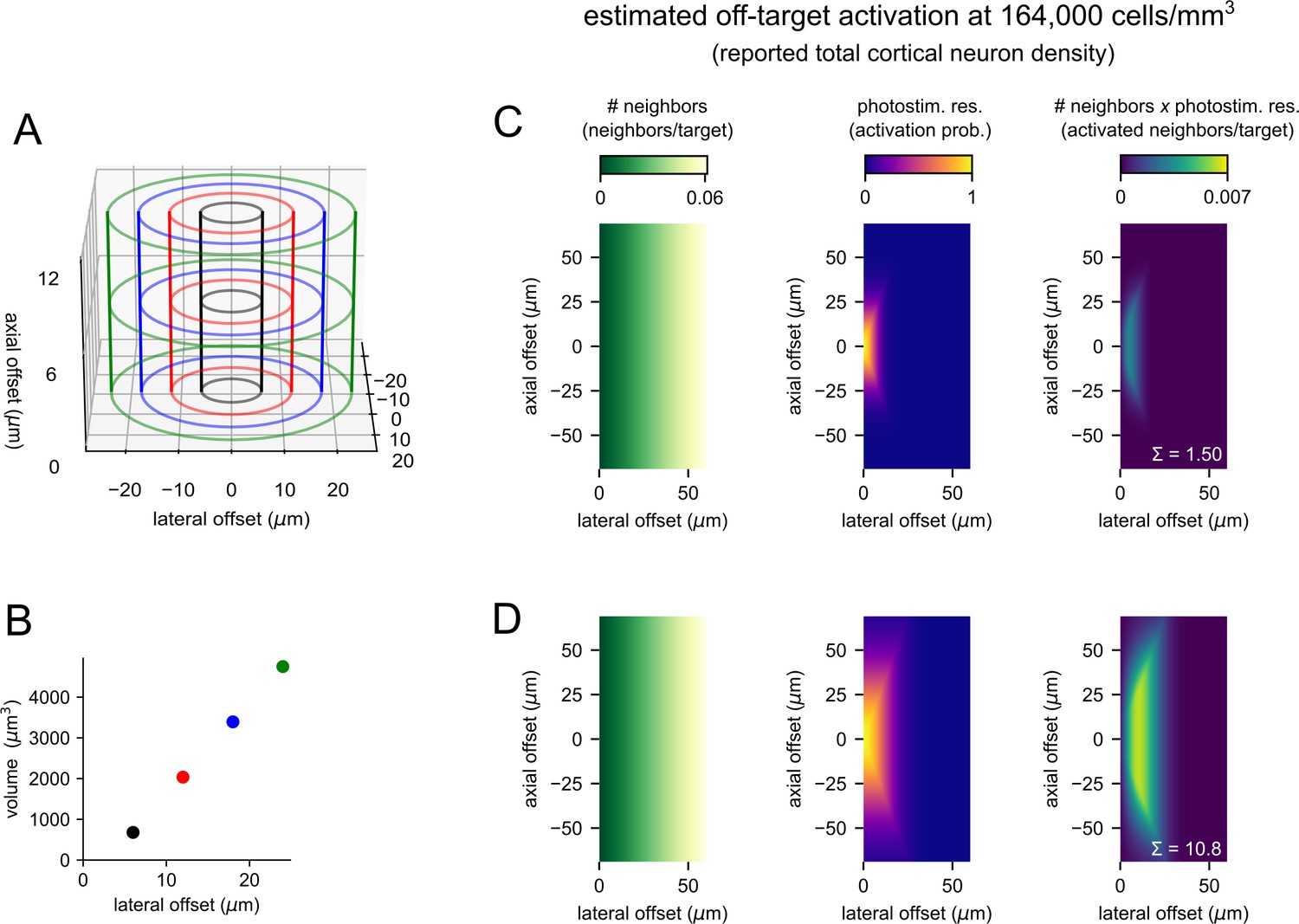
Estimation of off-target photostimulation.
(A) Illustration of bins used to measure the number of neighbors per cell with combined lateral and axial offsets (corresponding to two-dimensional histograms in Figure 2F and G). To avoid intersecting lines, the z-axis of this three-dimensional rendering was not drawn to scale. (B) The volume of each bin in panel (A) plotted against lateral offset (outer radius of the bin). Markers are colored to match panel (A). (C) Estimation of off-target activation using a high-resolution photostimulus with homogenously distributed photosensitive cells at a density of 164,000 cells/mm3. Panels follow the same schema as Figure 2F and G. Left panel: heatmap of the number of neighbors per cell at combined lateral and axial offsets. Middle panel: heatmap of the photostimulus resolution estimated using a lateral full-width at half-maximum (FWHM) = 12 µm and an axial FWHM = 35 µm. Right panel: heatmap of the number of activated off-target cells per targeted cell – estimated as the product of the number of neighbors and the probability of off-target activation. The sum across all distances (1.50; white text) estimates the average number of off-target cells activated by photostimulation. (D) Same as panel (C) for a relatively low-resolution photostimulus with a lateral FWHM = 24 µm and an axial FWHM = 66 µm. Analogous estimates were made for cellular densities from 10,000 to 164,000 cells/mm3 and are plotted as black and gray lines in Figure 2H.
Figure 3 with 3 supplements
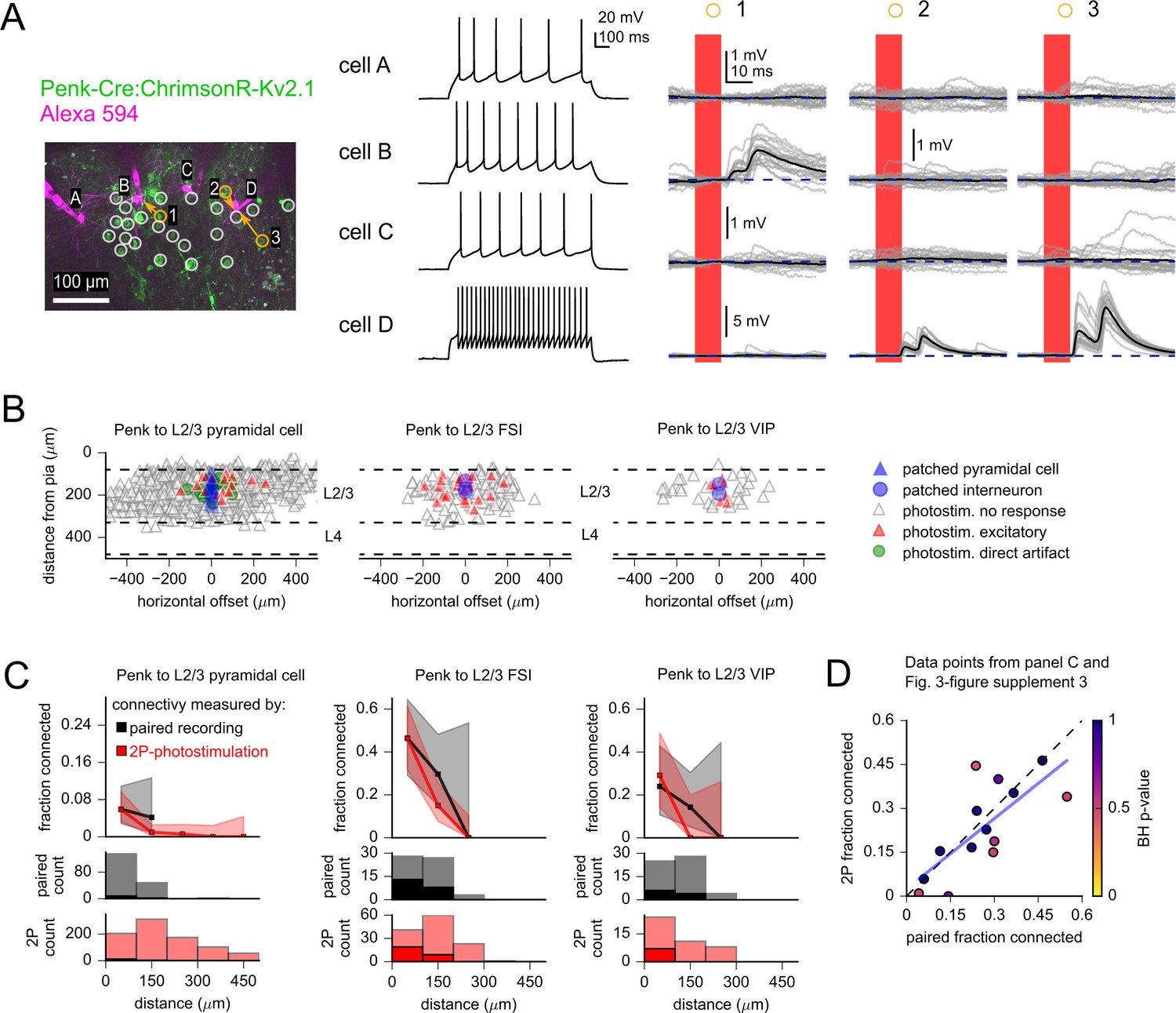
Measurement of intralaminar excitatory connectivity by two-photon optogenetic stimulation.
(A) Example experiment measuring connectivity from L2/3 excitatory neurons labeled by the Penk-Cre line to three L2/3 pyramidal cells (PCs) (cells A–C) and one fast-spiking interneuron (FSI) (cell D). Left: flattened z-stack of patched neurons filled with Alexa 594 (magenta) and EYFP signal from soma-targeted ChrimsonR-expressing neurons (green). Yellow circles: photostimulated cells with responses plotted in right panels. White circles: photostimulated cells with responses not shown. Middle: voltage responses to 1 s current injection, +40 pA relative to rheobase. Right: photoresponses to indicated locations. Photostimulation occurred during the red bar, black traces are an average of individual voltage responses (gray traces). The y-axis scale was increased for cell D to accommodate the large excitatory postsynaptic potentials (EPSPs). (B) Summary maps of Penk-labeled excitatory inputs to the indicated subclass of postsynaptic cell (n = 895 connections probed to L2/3 PCs, 125 to L2/3 FSIs, and 43 to L2/3 putative VIP interneurons). Locations of neurons are plotted according to their distance from the pia and the horizontal distance between cells with the following color scheme: blue, postsynaptic cells (n = 25 PCs, three FSIs, two putative VIP interneurons); gray, photostimulated neurons that did not evoke a synaptic response; red, photostimulated cells that produced an excitatory response; green, photostimulated cells that produced a direct stimulus artifact due to expression of ChrimsonR in a subset of the patched L2/3 PCs (19 photostimulus locations). Dashed lines represent approximate layer boundaries. Positive horizontal offsets correspond to presynaptic cells posterior to the postsynaptic cell. (C) Connection probability measured by two-photon optogenetic stimulation (red) or paired recording (black). Distance refers to total Euclidean distance in three dimensions. Shading represents 95% confidence intervals. Histograms on bottom rows indicate number of connections probed (faint colors) and identified (saturated colors) using each technique. (D) Connection probability measured by two-photon optogenetic stimulation plotted against corresponding measures made by paired recordings. Each point represents a category of connection defined by presynaptic and postsynaptic cell subclass and intersomatic distance. See Figure 3—figure supplement 3 and Table 1 for additional statistics. Color of markers indicates multiple-hypothesis-corrected p-values generated by performing a Fisher’s exact test for each dataset, followed by a Benjamini–Hochberg procedure with a false discovery rate set to 0.25. A high false discovery rate was used to avoid type II errors that could discount differences between the two techniques. Dashed line represents unity. Blue line represents a linear regression between the connection probabilities measured by each method (slope = 0.80 ± 0.21, y-intercept = 0.03 ± 0.06).
-
Figure 3—source data 1
Raw values for plots in Figure 3.
- https://cdn.elifesciences.org/articles/71103/elife-71103-fig3-data1-v2.xlsx
Figure 3—figure supplement 1
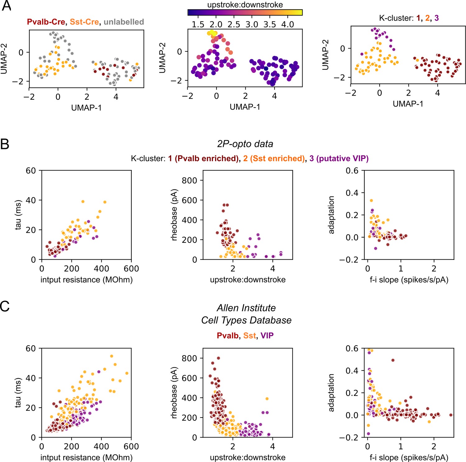
Classification of recorded interneurons using intrinsic electrophysiological features.
At the start of two-photon mapping experiments, 14 intrinsic electrophysiological properties were measured shortly after whole-cell break-in (see ‘Materials and methods’). (A) Left: data from 100 interneurons are plotted via a Uniform Manifold Approximation and Projection (UMAP) method (Becht et al., 2018). Of these cells, 27 were labeled by the Sst-Cre line (orange), 11 were labeled via the Pvalb-Cre line (maroon), and the remaining 62 were genetically unlabeled (gray). Unlabeled cells come from experiments in which an alternative Cre line was used to drive the expression of ChrimsonR (e.g., Penk-Cre, Rorb-Cre, Tlx3-Cre). Cells labeled by the Pvalb- and Sst- Cre lines are found on opposite sides of the UMAP. Middle: a cluster of unlabeled cells near the top of the UMAP displayed properties qualitatively consistent with known features of VIP-expressing interneurons (e.g., large upstroke:downstroke ratio). Right: based on genetic labeling and observed intrinsic properties, we hypothesized that groups in the data corresponded to Pvalb-, Sst-, and VIP-expressing subclasses of interneurons. Therefore, we applied K-means clustering with the number of clusters set to 3. Clustering was based on the first eight principal components (PCs) of the intrinsic parameters (these eight PCs explain 93% of the total variation). The resulting clusters were highly consistent with the UMAP visualization and partial genetic labeling. The first cluster (maroon) included all 11 Pvalb-labeled cells, 2 Sst-labeled cells, and 33 unlabeled cells. A second cluster (orange) contained the majority of the Sst-labeled cells (25/27) and 12 unlabeled neurons. A third cluster (purple) consisted entirely of unlabeled cells (16) and corresponded to the putative VIP-expressing neurons. Finally, we compared the intrinsic features of neurons in unsupervised clusters to genetically labeled interneurons in the Allen Institute Cell Types Database (Gouwens et al., 2019) (panels B and C). Recordings in these two datasets were made under different recording conditions (most notably, data from mapping experiments do not include blockers of synaptic transmission) and therefore the distributions of some parameters are shifted between the datasets. Despite this, the relative properties of the clusters in the two-photon mapping dataset are highly consistent with data from the Cell Types Database. For example, compared to Sst and VIP neurons, cells in the Pvalb cluster displayed lower input resistances, faster membrane time constants, more symmetrical spikes, and little adaptation of interspike intervals. These similarities combined with the accurate classification of the labeled Pvalb and Sst neurons impart a high degree of confidence in the accuracy of the clusters. We therefore used cluster membership to define subclasses of patched interneurons in two-photon mapping data.
-
Figure 3—figure supplement 1—source data 1
Raw values for plots in Figure 3—figure supplement 1.
- https://cdn.elifesciences.org/articles/71103/elife-71103-fig3-figsupp1-data1-v2.xlsx
Figure 3—figure supplement 2
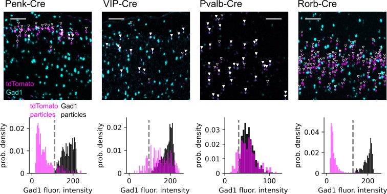
Estimation of interneuron labeling by the Penk-Cre driver line.
Top: pseudocolored example images of double fluorescence in situ hybridization (dFISH) staining for tdTomato (magenta) and Gad1 (cyan) mRNA from Ai14 reporter mice crossed to the indicated Cre lines. Scale bars = 100 µm. Inverted triangles are offset above all automatically detected particles in the tdTomato channel. Closed triangles indicate significant Gad1 fluorescence within the region of interest (ROI) defined by the tdTomato particle. Open triangles indicate tdTomato particles with Gad1 fluorescence below threshold. Bottom: normalized histograms showing the distribution of Gad1-associated fluorescence intensity within automatically determined ROIs for each Cre line. For each images, Gad1 fluorescence was measured in both tdTomato defined ROIs (magenta) and Gad1 defined ROIs (black). The threshold for classifying a tdTomato ROI as Gad1 positive was set to the minimum fluorescence intensity measured in automatically detected Gad1 ROIs within the same experiment (vertical dashed line). This threshold was set independently for each experiment to account for variability in fluorescence intensity (most notably in Pvalb-Cre). The fraction of tdTomato-labeled cells that were Gad1 positive was as follows: Penk: 26/211 cells, 12%; VIP: 191/255 cells, 85%; Pvalb: 208/243 cells, 86%; Rorb 13/455 cells, 2.9%.
Figure 3—figure supplement 3
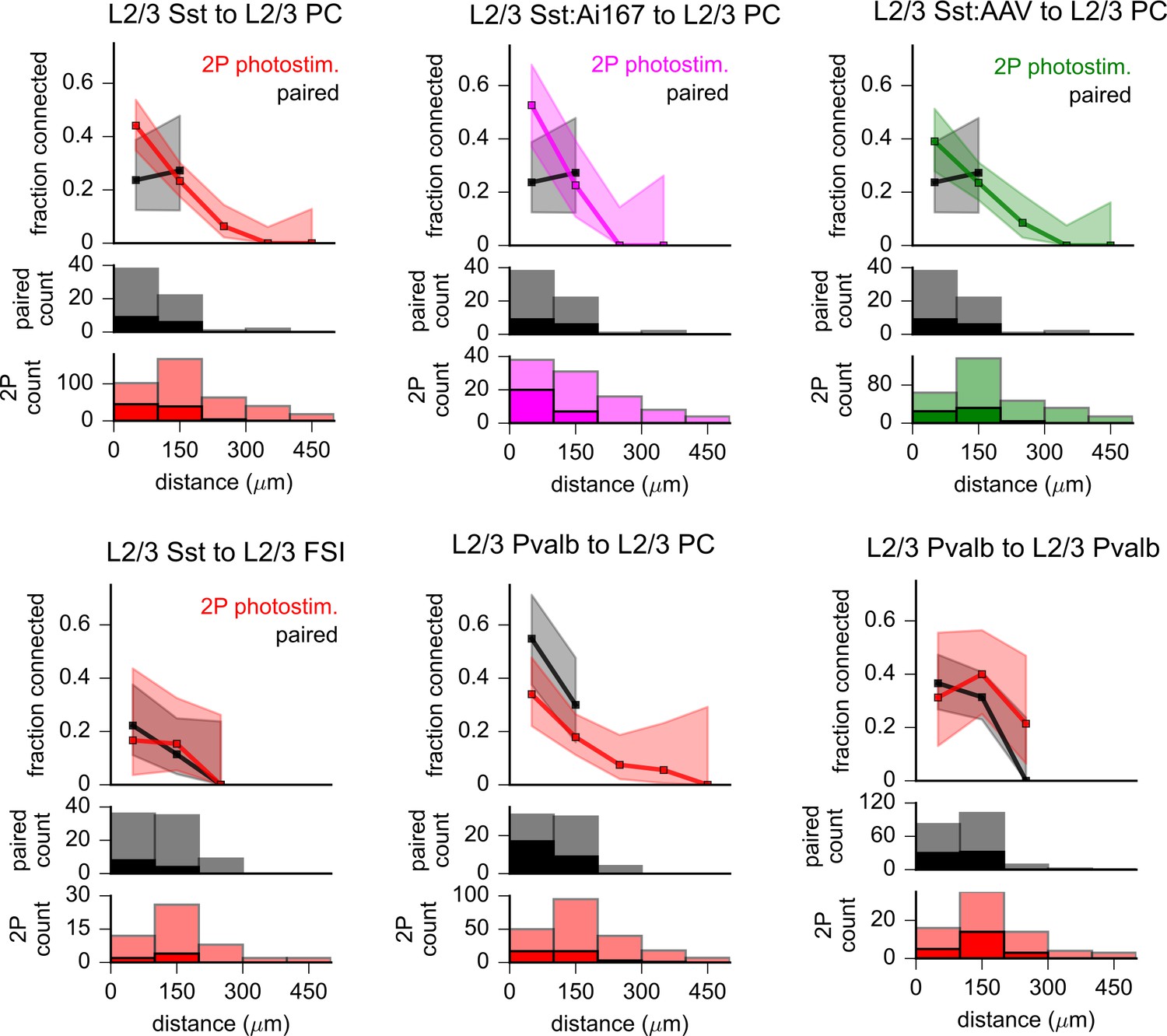
Comparison of intralaminar inhibition measured using two-photon optogenetics to paired recordings.
The fraction of probed connections that indicated a synaptic response as measured by paired recording (black) or using two-photon optogenetic stimulation (colors). Shading represents 95% confidence intervals. Histograms on bottom rows indicate the number of connections probed (faint colors) and identified (saturated colors) using each technique. In all plots, distance was calculated as the total Euclidean distance in three dimensions. The graph labeled ‘L2/3 Sst to L2/3 PC’ represents pooled data acquired using Sst-Cre with either Ai167 or adeno-associated virus (AAV)-mediated opsin expression. In adjacent panels, Sst photostimulation data are split according to expression method (see labels). While connectivity from L2/3 Sst to L2/3 pyramidal cell (PC) within 100 µm was higher with Ai167 than with AAV, this difference was not statistically significant (Sst:Ai167: 53%, 20 connections/38 probed; Sst:AAV: 39%, 25 connections/64 probed; p=0.22, Fisher’s exact). Pooled photostimulation data were used for comparison to paired recordings in Figure 3D and in Table 1 to increase the statistical power of the comparison. L2/3 Sst to L2/3 fast-spiking interneuron (FSI), L2/3 Pvalb to L2/3 PC, and L2/3 Pvalb to L2/3 Pvalb datasets were collected using only AAV-mediated opsin expression.
Figure 4 with 1 supplement

Measurement of excitatory connectivity from Rorb-labeled neurons to L2/3 pyramidal cells (PCs).
(A) Example experiment measuring connectivity to a L2/3 PC from excitatory neurons labeled using Rorb-Cre:Ai167. Panel i: synaptic responses evoked by photostimulation of a Rorb-labeled cell (photostim. 1) Image of ChrimsonR-tdT signal (bottom) was captured immediately prior to photostimulation. Panel ii: the cell targeted by photostimulus 1 was subsequently patched and synaptic responses (top) were evoked by suprathreshold current injection into the Rorb-neuron. Image of the Rorb-labeled cell filled with Alexa 488, captured at the end of the experiment (bottom). Panel iii: additional photostimulus responses including a smaller excitatory synaptic response (photostim. 4). Overview images of photostimulated and patched cells collected at the end of the experiment (bottom). Dashed green lines represent original location of the postsynaptic recording pipette (removed before collection of the z-stack). Blue inset corresponds to location of images from panels i and ii. In all panels, black traces are an average of individual sweeps (gray traces). (B) Summary maps for all experiments with Rorb-Cre mice crossed to Ai167 (left) or injected with adeno-associated virus (AAV) encoding soma-targeted ChrimsonR (right; n = 2,269 connections probed using Rorb:Ai167, 1157 connections probed using Rorb:AAV). Locations of neurons are plotted with the following color scheme: black, postsynaptic L2/3 PCs (n = 79 recordings using Rorb:Ai167, 28 recordings using Rorb:AAV); gray, photostimulated neurons that did not evoke a synaptic response; magenta/green, photostimulated cells that produced an EPSP using Ai167 or AAV-mediated ChrimsonR expression. Dashed lines represent approximate layer boundaries. Positive horizontal distances correspond to presynaptic cells posterior to the postsynaptic cell. (C, left) The fraction of Rorb-labeled neurons connected to L2/3 PCs plotted against the distance of the presynaptic cell from the pia. Measurement was limited to cells within 300 µm horizontal distance. Shading indicates 95% confidence intervals. The fraction of cells connected, and associated confidence intervals, were not drawn if fewer than 20 connections were probed within a distance bin. Right: histogram of number of connections probed within each distance bin using either Ai167 or AAV, within 300 µm horizontal distance.
-
Figure 4—source data 1
Raw values for plots in Figure 4.
- https://cdn.elifesciences.org/articles/71103/elife-71103-fig4-data1-v2.xlsx
Figure 4—figure supplement 1
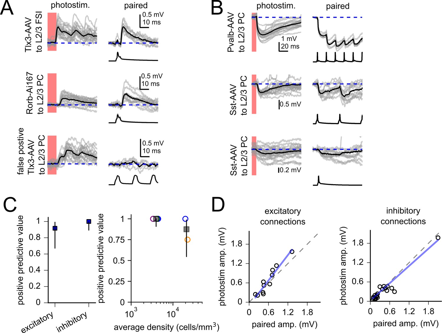
Verification of optically identified connections.
(A) Examples of verification experiments using excitatory Cre lines. Left panels display individual two-photon-evoked synaptic responses (gray) and the average responses (black). Right panels display synaptic responses evoked by current injection into the same presynaptic cell. Presynaptic spikes are plotted below postsynaptic traces. The top two panels were confirmed connections, the bottom panel represents the single false positive identified in these experiments (from 12 recordings of optically identified excitatory presynaptic partners). Broken down by Cre line and expression method, results testing excitatory connections were as follows: Rorb-Ai167: four confirmed/four tested (filled blue circle in panel C), Rorb-AAV: four confirmed/four tested (open blue circle), Tlx3-AAV: three confirmed/four tested (open orange circle). (B) Same as panel (A) for inhibitory connections. All 22 optically identified inhibitory synaptic connections tested were confirmed. Broken down by Cre line, results testing inhibitory connections were as follows: Sst-AAV: 15 confirmed/15 tested (open green circle in panel C), Pvalb-AAV: seven confirmed/seven tested (open purple circle). (C, left) Positive predictive value (number of confirmed connections/number of tested connections) for excitatory and inhibitory Cre lines. Error bars represent 95% confidence intervals. Right: positive predictive value for each experimental condition plotted against the average density of labeled neurons (circles). Data were binned as either low-density experiments (Rorb:Ai167, Pvalb:AAV, Sst:AAV) or high-density experiments (Rorb:AAV, Tlx3:AAV); positive predictive values and associated confidence intervals for each category are represented as gray squares and vertical lines. (D) Amplitudes of postsynaptic potentials (PSPs) measured in response to two-photon stimulation versus amplitudes of PSPs measured by paired recordings. Dashed lines represent unity. Blue lines represent linear regression of the two PSP measurements. Amplitudes were strongly correlated for both excitatory (Pearson’s R = 0.95, p=6.2 e-6) and inhibitory connections (Pearson’s R = 0.96, p=1.2 e-12). Connections were initially tested by 50 Hz current injection into the presynaptic cell. The frequency of current injection was then lowered (20–5 Hz) for further characterization. In some cases, one of the recordings failed before using lower-frequency current injection. Amplitude measurements from paired recordings were made from the first PSP of the lowest stimulation frequency available. First PSP amplitudes were similar for connections tested at multiple frequencies.
Figure 5 with 3 supplements
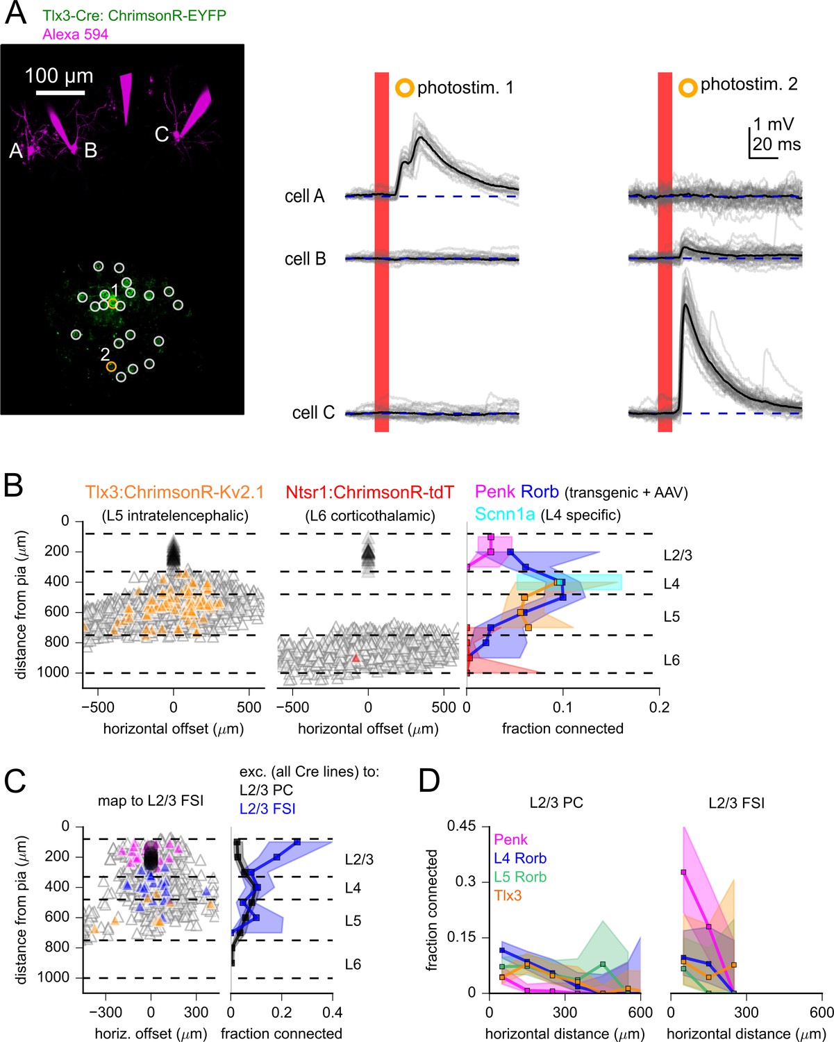
Measurement of translaminar excitatory connectivity to L2/3.
(A) Example experiment measuring connectivity from Tlx3-labeled excitatory neurons to three L2/3 pyramidal cells (PCs) (cells A–C). Left: flattened z-stack of recorded L2/3 PCs filled with Alexa 594 (magenta) and EYFP signal from soma-targeted ChrimsonR-expressing neurons (green). Yellow circles: photostimulated cells with responses plotted in the adjacent panels. White circles: photostimulated cells with responses not shown. Right: responses to photostimulation. Photostimulus occurred during the red bar, black lines are an average of individual sweeps (gray). (B) Summary maps for experiments with Tlx3-Cre (left, n = 1734 connections probed) and Ntsr1-Cre (center, n = 1145 connections probed) mice. Locations of neurons are plotted according to their distance from the pia and the horizontal distance between cells with the following color scheme: blue, postsynaptic L2/3 PCs (Tlx3 n = 46, Ntrs1 n = 23); gray, photostimulated neurons that did not evoke a synaptic response; orange/red, stimulated cells that produced an EPSP using Tlx3-Cre or Ntsr1-Cre. Dashed lines represent approximate layer boundaries. Positive horizontal distances correspond to presynaptic cells posterior to the postsynaptic cell. Right: the measured connection probability plotted against the distance of the presynaptic cell from the pia to L2/3 PCs for the indicated Cre lines. (C, left) Summary map for experiments measuring excitatory inputs to L2/3 fast-spiking interneurons (FSIs) using either Penk (magenta), Rorb (blue), or Tlx3 (orange) Cre lines to drive opsin expression (n = 648 connections probed, 63 connections found, from 19 postsynaptic recordings). Right: the connection rate of excitatory neurons to L2/3 PCs (black) and L2/3 FSIs (blue). Data across excitatory Cre lines were pooled in this plot. Measurement of connection rate versus pia distance was limited to cells < 300 µm horizontal distance (panels B and C). (D) Connection rate plotted against the absolute value of the horizontal distance between pre- and postsynaptic neurons for the indicated Cre lines to either L2/3 PCs (left) or L2/3 FSIs (right). Shading indicates 95% confidence intervals in panels (B) – (D). The connection probability and associated confidence intervals were not drawn if fewer than 20 connections were probed within a distance bin.
-
Figure 5—source data 1
Raw values for plots in Figure 5.
- https://cdn.elifesciences.org/articles/71103/elife-71103-fig5-data1-v2.xlsx
Figure 5—figure supplement 1
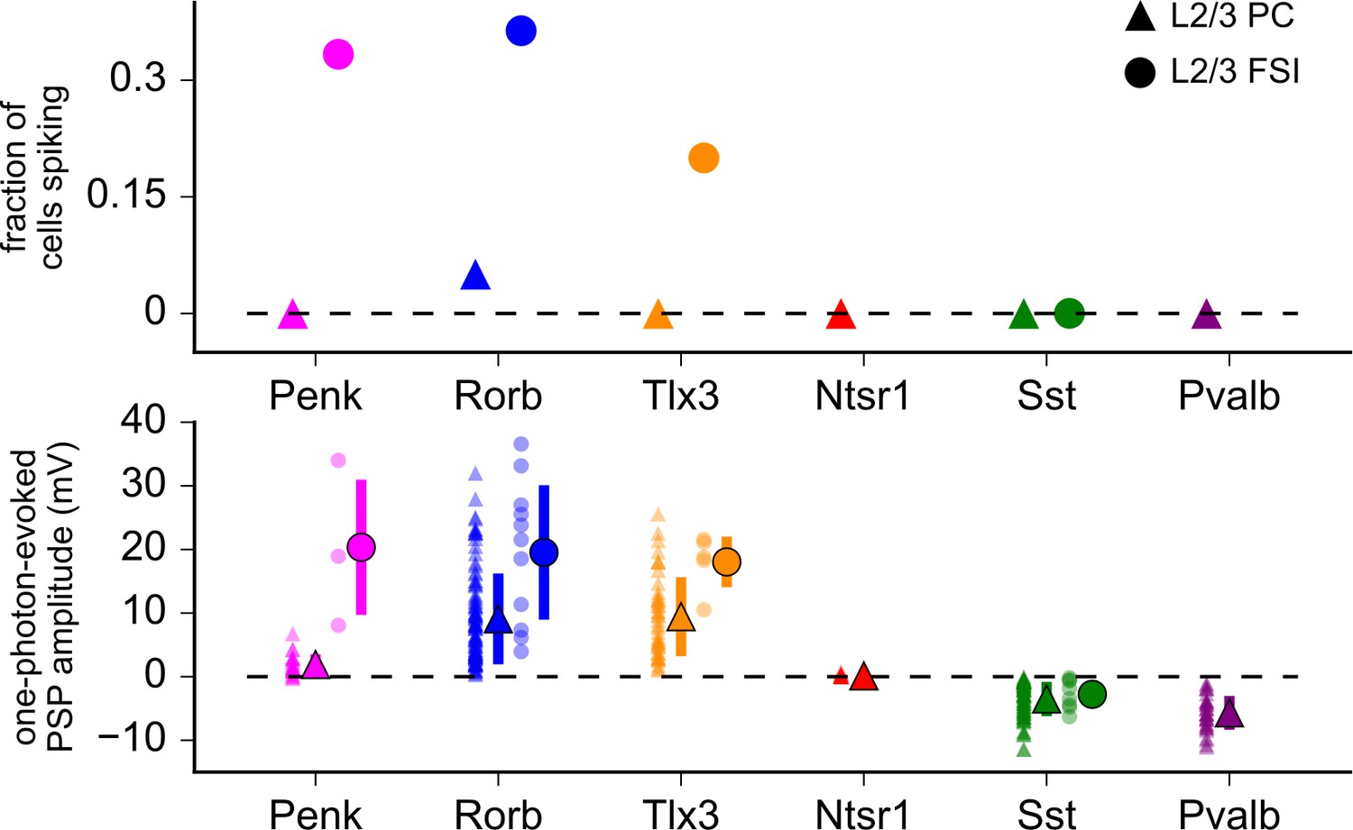
One-photon-evoked synaptic responses.
Top: the fraction of cells generating action potentials (APs) in response to one-photon stimulation. Bottom: amplitudes of one-photon-evoked postsynaptic responses. Data were collected from the same postsynaptic cells used for two-photon mapping. Responses were measured following a single 1 ms photostimulus (590 nm) via a ×40 objective centered over the patched cell (triangles: L2/3 pyramidal cells [PCs]; circles: L2/3 fast-spiking interneurons [FSIs]). In a subset of experiments using Tlx3-Cre and Ntsr1-Cre, responses were also measured with the objective centered over the primary presynaptic layer labeled by each Cre line (L5 and L6, respectively). Photoresponses were similar to those collected over L2/3, presumably a result of the robustness of full-field one-photon stimulation and its capacity to directly excite axons. Small, transparent markers in the bottom panel represent values for individual neurons. Large, opaque makers indicate mean ± SD. In some cases, error bars are smaller than the marker. In experiments using Penk, Rorb, or Tlx3 driver lines, a subset of recorded cells generated APs (more common in FSIs than in PCs). For these cells, the one-photon-evoked response was measured as the difference between AP threshold and the resting membrane potential. Recordings from ChrimsonR-expressing cells in the Penk and Pvalb Cre lines are not included in this analysis as we are unable to distinguish direct photostimulation (ChrimsonR-mediated depolarization) and synaptic responses.
Figure 5—figure supplement 2
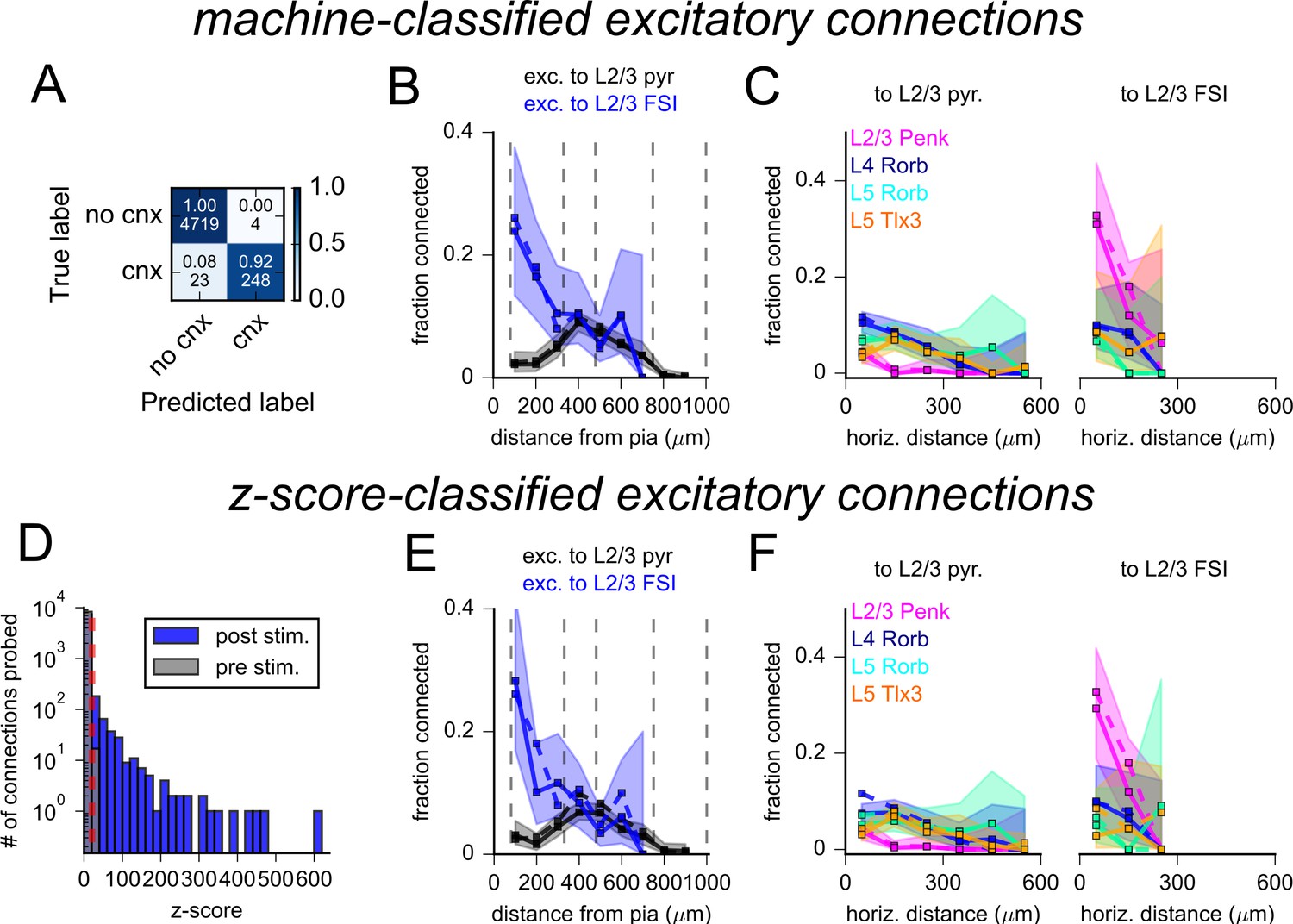
Evaluation of excitatory connectivity.
(A) Confusion matrix describing the results of a support vector machine tested on 4994 photostimulus responses. The top numbers within each element represent the fraction of photoresponses classified by the support vector machine (SVM) as containing an excitatory response (cnx) or not (no cnx). Bottom values are corresponding counts. (B) Connection probability versus the distance of the presynaptic neuron from the pia measured for L2/3 pyramidal cells (PCs) (black) and L2/3 fast-spiking interneurons (FSIs) (blue). Sold lines and shading represent connection probability as determined by the SVM. Dashed lines represent connection probability determined by human annotation (replotted from Figure 5C). (C) Connection probability versus horizontal distance between neurons for cells of the indicated layer and Cre-line label. Data are split by the subclass of the postsynaptic cell (left: L2/3 PCs; right: L2/3 FSIs). Connection probabilities measured by human annotation are replotted from Figure 5D as dashed lines. Solid lines represent connectivity determine by machine classification of the same data. (D) Histograms of maximum voltage responses normalized to background variance (z-score) measured 50 ms after photostimulation (post-stimulus, blue) or in a 50 ms window preceding photostimulation (pre-stimulus, gray). Tested pairs were classified as connected if the post-stimulus z-score exceeded the 99th percentile of all pre-stimulus z-scores (red dashed line). (E) Connection probability versus distance from the pia (as in panel B) with connected cells classified by z-scores. (F) Connection probability versus the horizontal distance between neurons (as in panel C) with connected cells classified by z-scores. Shading throughout the figure represents 95% confidence intervals.
Figure 5—figure supplement 3
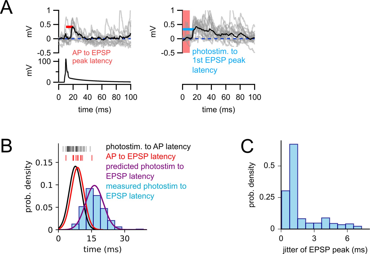
The timing of two-photon-evoked excitatory responses is consistent with monosynaptic connectivity.
(A) Left panel: example experiment illustrating the measurement of action potential (AP) to EPSP peak latency (red line) from a confirmed excitatory connection (Rorb-Cre with adeno-associated virus (AAV)-mediated ChrimsonR expression to a L2/3 pyramidal cell [PC]). Analogous measures were made from all 11 confirmed excitatory connections (vertical red markers in panel B). Right panel: two-photon-evoked responses for the same connection, recorded before patching of the presynaptic cell. Light blue line: the latency measured from the start of the photostimulus to the first detected EPSP peak. This measure was collected for all optically identified excitatory connections (light blue histogram in panel B). (B) Vertical black markers: latencies from photostimulus onset to the first light-evoked AP for the excitatory Cre lines (measured from cell-attached characterization experiments, Figure 1). Black curve: Gaussian probability density function (PDF) fit to these latencies. Red vertical bars: AP to EPSP latencies measured from confirmed excitatory connections (as illustrated in panel A). Red curve: Gaussian PDF fit to these latencies. Purple curve: predicted distribution of photostimulus to EPSP latencies, generated by convolving the two measured PDFs (photostimulus to AP and AP to EPSP) to estimate the expected distribution of the sum of these two latencies. Light blue bar plot: histogram of the measured distribution of photostimulus to EPSP latencies for optically identified connections from excitatory Cre lines. The similarity of the predicted (purple) and measured (blue) distributions demonstrates that the observed latencies of optically identified responses are consistent with the underlying connections being monosynaptic. Estimation of the predicted photostimulus to EPSP latencies (purple curve) assumes the two underlying latencies are independent and each reasonably well-described by Gaussian distributions. Alternatively, one could consider the sum of the largest observed latencies (sum: 29.6 ms; photostimulus to AP: 14.4 ms, AP to EPSP peak: 15.2 ms) to define a window of acceptance and reach a similar conclusion. (C) Histogram of optically evoked EPSP jitter. Jitter was typically higher than that of light-evoked APs (Figure 1); however, this is likely due to the greater variability in EPSP waveforms compared to highly stereotyped APs, as well as the presence of spontaneous background synaptic activity.
Figure 6 with 2 supplements
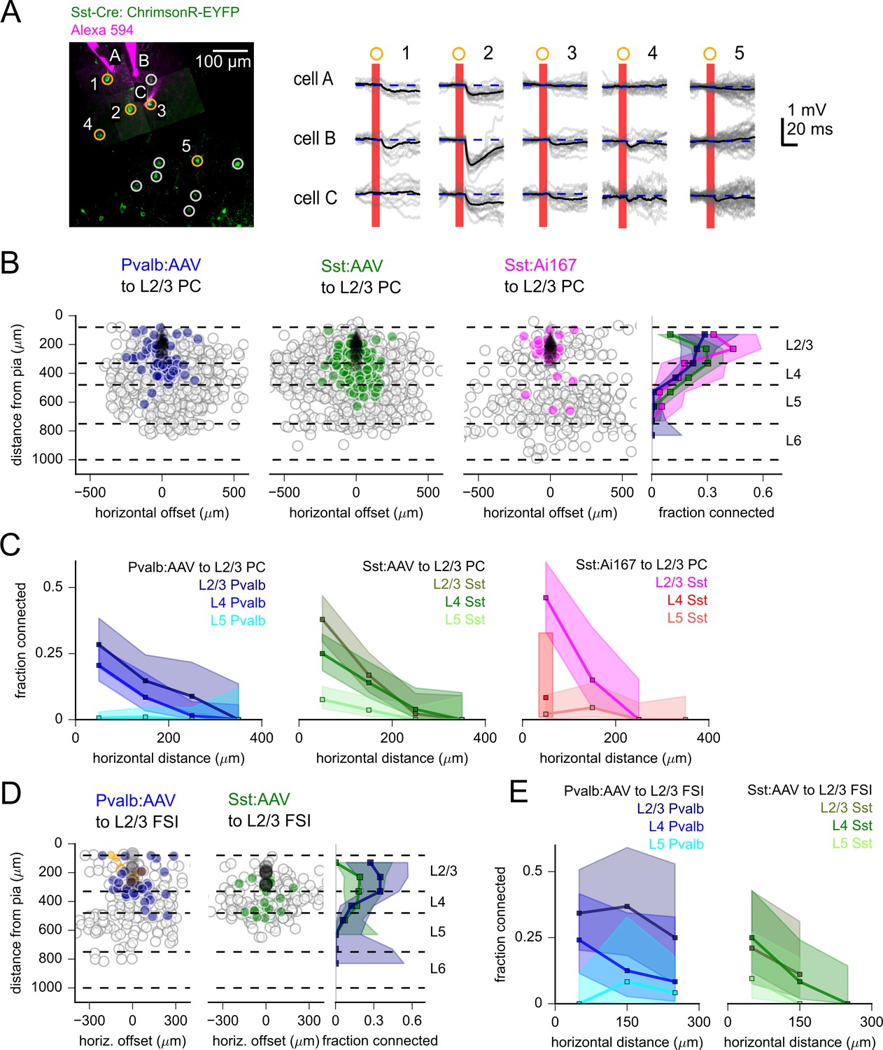
Measurement of inhibitory connectivity to L2/3 pyramidal cells (PCs).
(A) Example experiment measuring connectivity from Sst neurons to three L2/3 PCs (cells A–C). Left: flattened z-stack of recorded L2/3 PCs filled with Alexa 594 (magenta) and EYFP signal from soma-targeted ChrimsonR-expressing neurons (green). Yellow circles: photostimulated cells with responses plotted in right panels. Responses following stimulation of cells in white circles are not shown. Right: responses to photostimulation of the indicated cells. Postsynaptic cells were depolarized to –55 mV with automated bias current to increase the driving force of inhibitory currents. Photostimulation occurred during the red bar, black lines are an average of individual sweeps (gray). (B) Summary maps of inhibitory connections to L2/3 PCs for experiments with Pvalb:AAV-injected (902 connections probed, 33 postsynaptic recordings), Sst:AAV-injected (1052 connections probed, 49 postsynaptic recordings), and Sst:Ai167 mice (360 connections probed, 39 postsynaptic recordings). Locations of neurons are plotted according to their distance from the pia and the horizontal distance between cells with the following color scheme: black, postsynaptic L2/3 PCs; gray, photostimulated neurons that did not evoke a synaptic response in the recorded cell; blue/green/magenta, stimulated cells that produced an IPSP using Pvalb-Cre:AAV/Sst-Cre:AAV/Sst:Ai167-mediated ChrimsonR expression. Dashed lines represent approximate layer boundaries. Positive horizontal offsets correspond to presynaptic cells posterior to the postsynaptic cell. Right: measured connection probability plotted against the distance of the presynaptic cell from the pia for the three datasets. Measurement of connection probability versus pia distance was limited to cells < 200 µm horizontal distance. (C) Connection probability versus horizontal distance between pre- and postsynaptic cells for each dataset, separated by the cortical layer of the presynaptic cell. (D) Summary maps of inhibitory connections to L2/3 fast-spiking interneurons (FSIs) (Pvalb: 201 connections probed, 12 postsynaptic recordings; Sst: 166 connections probed, 7 postsynaptic recordings) following the same scheme as panel (B), with the addition of orange markers to indicated stimulus locations that produced a direct stimulus artifact due to expression of ChrimsonR in the patched, Pvalb-labeled neurons (13 photostimulus locations). Shading in panels (B) – (F) represents 95% confidence intervals. The fraction of cells connected and associated confidence intervals were not drawn if fewer than 10 connections were probed within a distance bin.
-
Figure 6—source data 1
Raw values for plots in Figure 6.
- https://cdn.elifesciences.org/articles/71103/elife-71103-fig6-data1-v2.xlsx
Figure 6—figure supplement 1
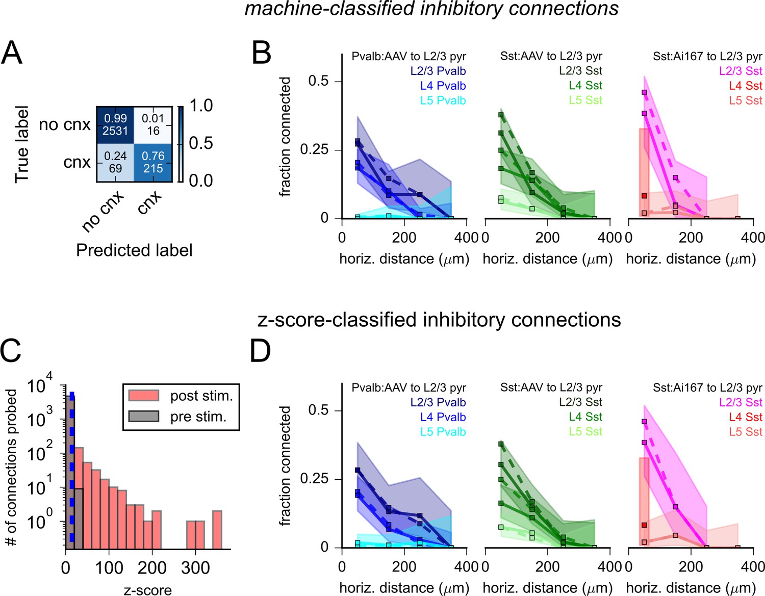
Evaluation of inhibitory connectivity.
(A) Confusion matrix describing the results of a support vector machine (SVM) tested on 2831 photostimulus responses. The top numbers within each element represent the fraction of human-annotated photoresponses classified by the SVM as containing or not containing an inhibitory synaptic response (labeled cnx or no cnx, respectively). Bottom values are corresponding counts. (B) Connection rate versus horizontal distance between pre- and postsynaptic cells for each dataset, separated by the presynaptic cell’s layer of origin. Dashed lines represent connectivity as determined by human annotation (replotted from Figure 6C). Solid lines and shading represent machine classification of the same data. (C) Histograms of maximum voltage responses normalized to background variance (z-score) measured 50 ms after photostimulation (post-stimulus, red) or in a 50 ms window preceding photostimulation (pre-stimulus, gray). Cells were considered connected if the post-stimulus z-score exceeded the 99th percentile of all pre-stimulus z-scores (blue dashed line). (D) Connection probability versus horizontal distance between cells (as in panel B) with connected cells classified by z-scores indicated by solid lines. Shading represents 95% confidence intervals.
Figure 6—figure supplement 2
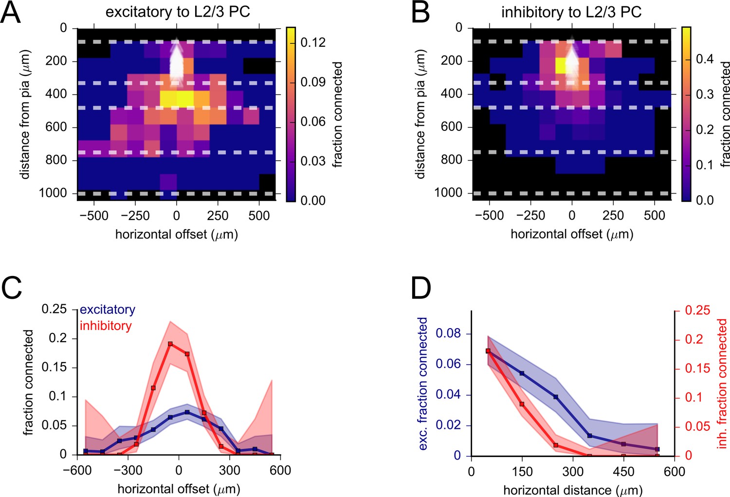
Spatial distribution of excitatory and inhibitory connectivity to L2/3 pyramidal cell (PCs).
(A) Heatmap of excitatory connection probability measured by pooling data from all excitatory Cre lines. White triangles indicate the locations of postsynaptic cells. Bin size was 100 μm × 100 μm. Black squares correspond to bins with fewer than 10 connections probed. Dashed lines represent approximate layer boundaries. (B) Heatmap of inhibitory connectivity measured by pooling data from Pvalb and Sst-Cre lines, as in panel (A). (C) Excitatory and inhibitory connectivity plotted against horizontal offset (positive values correspond to the presynaptic cell being posterior to the postsynaptic cell). (D) Excitatory and inhibitory connectivity plotted against horizontal distance (absolute value of the horizontal offset). Vertical axes for each plot were scaled to highlight a more gradual decline of excitatory connectivity. See Figures 4D and 5C for similar plots with presynaptic cells separated by Cre line and cortical layer. Shaded regions in panels (C) and (D) correspond to 95% binomial confidence intervals.
Figure 7 with 3 supplements
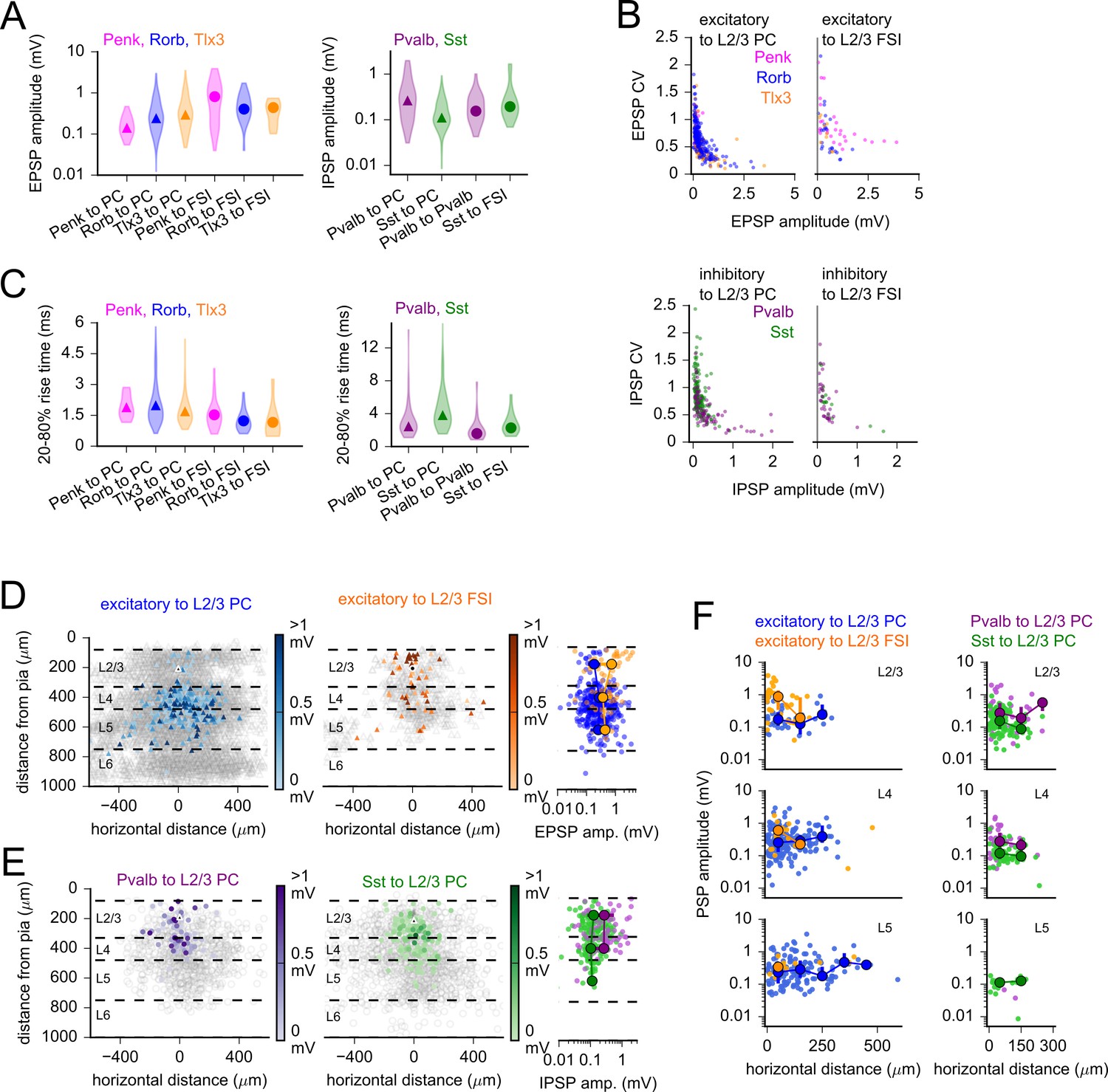
Postsynaptic potential (PSP) properties across subclasses and space.
(A) Violin plots of PSP amplitude distributions for excitatory (left) and inhibitory (right) Cre lines. Markers represent median values. (B) Coefficient of variation (CV) plotted against mean PSP amplitude for all connections of indicated subclass. Excitatory to L2/3 pyramidal cell (PC): Spearman’s R = –0.76, p=5e-67; excitatory to L2/3 fast-spiking interneuron (FSI): R = –0.58, p=1.2e-6; inhibitory to L2/3 PC: R = –0.65, p=7.2e-30; inhibitory to L2/3 FSI: R = –0.79, p=2.2e-12. (C) Violin plots of PSP rise time distributions for excitatory (left) and inhibitory (right) Cre lines. Markers represent median values. (D, left) Heatmaps of measured EPSP amplitudes plotted according to horizontal distance between cells and the distance of the presynaptic neuron from the pia. Dashed lines represent approximate layer boundaries. Black markers represent the average location of all postsynaptic cells. Right: EPSP amplitudes plotted against the distance of the presynaptic neuron from the pia. Larger markers represent median values for data binned by layer (markers are not drawn if fewer than three connections were measured within a distance bin). Error bars represent interquartile ranges (25–75% of data in each distance bin). Some error bars are smaller than the markers. (E) Same as panel (D) for the labeled inhibitory connection classes. (F) PSP amplitudes versus horizontal distance between cells for the indicated subclasses of excitatory (left) and inhibitory (right) connections. Plots are separated by the layer of origin of the presynaptic cell (see labels in top-right corners of each plot). Larger markers represent median and interquartile ranges as described for panel (D). Bin width is 100 µm.
-
Figure 7—source data 1
Raw values for plots in Figure 7.
- https://cdn.elifesciences.org/articles/71103/elife-71103-fig7-data1-v2.xlsx
Figure 7—figure supplement 1
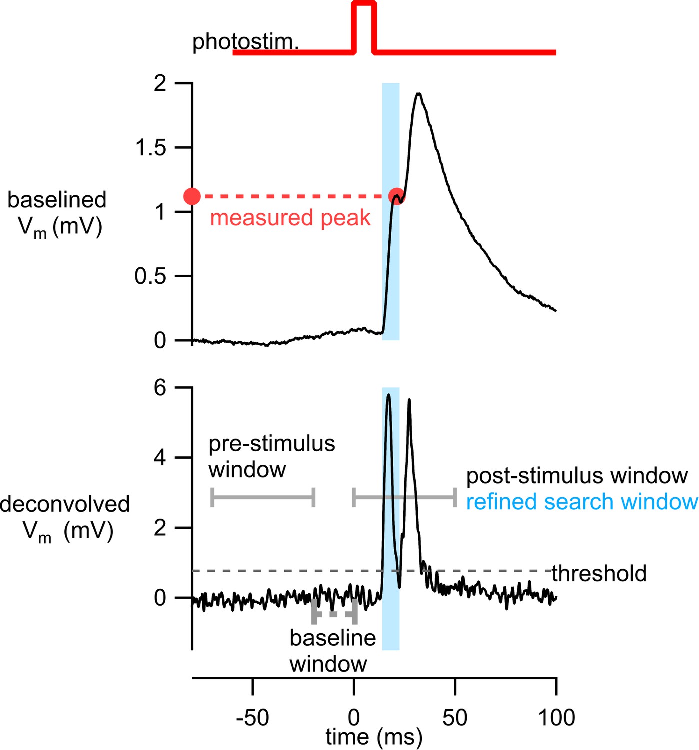
Strategy for measuring first response peak from photoresponses with multiple postsynaptic potentials (PSPs).
Example of an average membrane potential response from stimulation of a Tlx3 neuron (replotted from Figure 5A, photostim. 1 to cell A). The deconvolved membrane potential was generated using Equation 2. An initial response window from 0 to 50 ms was used to identify timing of PSPs and establish a refined search window (light blue) in which to measure the peak voltage response in the original trace. See ‘Analysis of PSP amplitudes’ for further details.
Figure 7—figure supplement 2
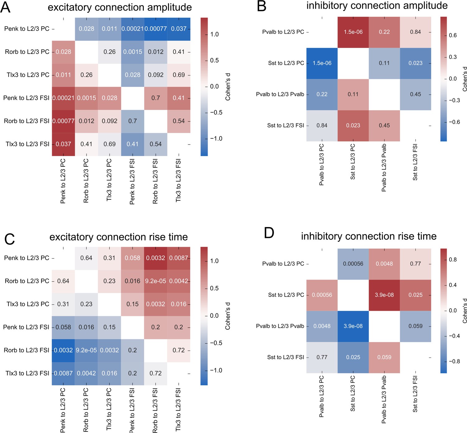
Statistical comparisons of postsynaptic potential (PSP) properties.
(A) Cohen’s d effect sizes comparing the distributions EPSP amplitudes of each connection class to all other connection classes. A Kruskal–Wallis (KW) test performed across all groups generated a p-value=2.1e-5. Numbers in each element are p-values from post hoc Dunn’s test for each comparison. (B) Same as panel (A) for IPSP amplitudes. KW p-value=1.3e-6. (C) Same as panel (A) for EPSP rise times. KW p-value=1.3e-6. (D) Same as panel (A) for IPSP rise times. KW p-value=4.4e-9.
Figure 7—figure supplement 3
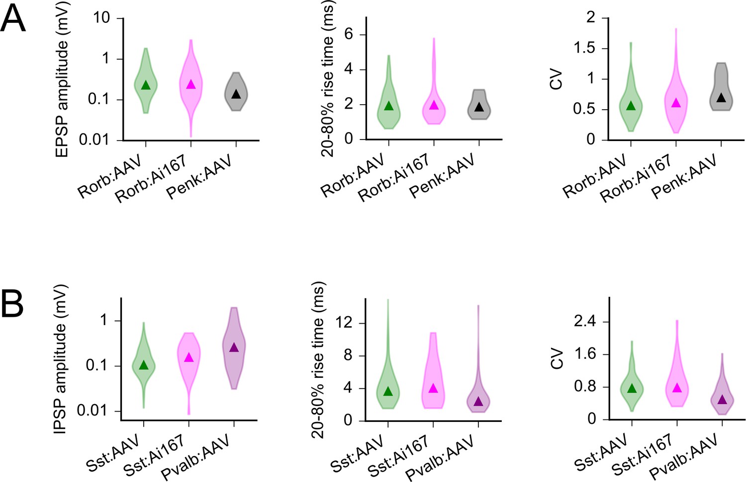
Comparison of postsynaptic potential (PSP) properties by opsin expression method.
(A) Violin plots (shaded distributions) and median values (triangles) for EPSP amplitude, rise time, and variability as measured in L2/3 pyramidal cells (PCs) from Rorb:AAV, Rorb:Ai167, and Penk:AAV experiments. Data from Penk-Cre are replotted from Figure 7 to illustrate greater differences across Cre lines than across expression strategies. Comparison of Rorb:AAV to Rorb:Ai167 amplitude: p=0.41, rise time: p=0.46, coefficient of variation (CV): p=0.39. (B) As in panel (A) for Sst:AAV, Sst:Ai167, and Pvalb:AAV. Comparison of Sst:AAV to Sst:Ai167 amplitude: p=0.23, rise time: p=0.41, CV: p=0.41. p-values are results of Mann–Whitney U tests following a Benjamini–Hochberg correction for multiple comparisons (for the six comparisons reported in this figure) with a false discovery rate = 0.1.
Figure 8 with 1 supplement
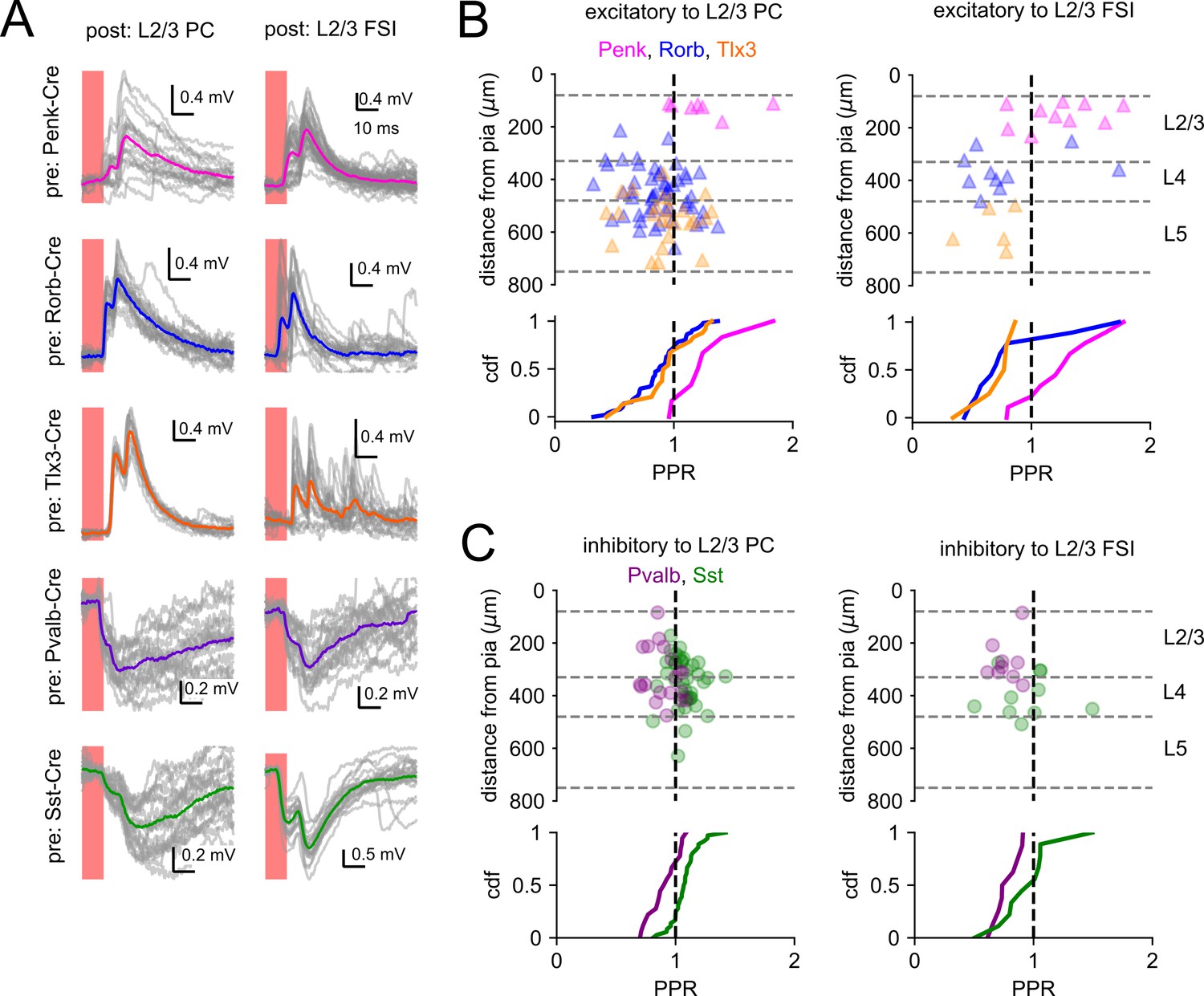
Short-term plasticity of optically evoked synaptic responses.
(A) Examples of light-evoked synaptic responses measured from indicated presynaptic Cre lines (rows) and postsynaptic subclasses (columns). Horizontal scale bar is set to 10 ms in all panels. Vertical scale was adjusted to accommodate the amplitude of each photoresponse. Individual photoresponses are plotted in gray, and average responses are represented by colored traces. (B) Top: paired-pulse ratio (PPR) of excitatory connections plotted according to the distance of the presynaptic cell from the pia. The colors of markers indicate the presynaptic Cre line. The vertical dashed line corresponds to a PPR = 1. The horizontal dashed lines represent approximate layer boundaries. Bottom: cumulative distribution function (CDF) of PPR values measured for each Cre line. (C) PPR values measured from inhibitory synapses as in panel (B).
-
Figure 8—source data 1
Raw values for plots in Figure 8.
- https://cdn.elifesciences.org/articles/71103/elife-71103-fig8-data1-v2.xlsx
Figure 8—figure supplement 1
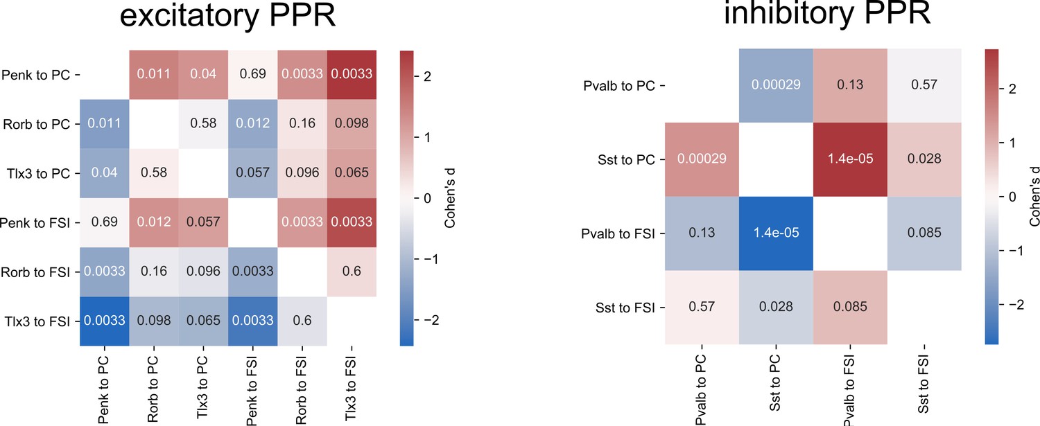
Statistical comparisons of paired-pulse ratios (PPRs).
Cohen’s d effect sizes comparing the distributions of PPRs measured for excitatory (left panel) and inhibitory (right panel) connections. A Kruskal–Wallis (KW) test comparing PPRs across excitatory groups generated a p-value=1.6e-4. For inhibitory groups, KW p-value=9.2e-7. Numbers in each element are p-values from a post hoc Dunn’s test for each comparison.
Figure 9 with 2 supplements

Convergence of synaptic inputs.
(A) All identified instances of convergent inputs to L2/3 pyramidal cells (PCs) from Penk (magenta), Rorb (blue), Tlx3 (orange), Pvalb (purple), or Sst (green)-labeled neurons. The same colors are used to indicate presynaptic Cre lines throughout the figure. Lines are drawn from identified presynaptic partners to a common point representing the L2/3 PC (triangle). Cases of convergence are ordered according to the distance of the postsynaptic cell from the pia. Dashed lines represent approximate layer boundaries. Scale bar = 200 µm. (B, left) Cartoon of completed convergence analysis. We identified all ordered pairs of photostimulated neurons (cell i and cell j, green) that shared a common potential postsynaptic partner (patched cell, gray). We further required that the first photostimulated cell (cell i) formed a connection to the postsynaptic cell (solid arrow). From these potential convergence motifs, we measured the probability that the second photostimulated cell (cell j) also forms a connection with the recorded postsynaptic cell. Middle: for excitatory Cre lines, the probability that cell j completes a convergence motif (Pj|i) plotted against the horizontal distance between photostimulated cells. Right: same as middle panel for inhibitory Cre lines. Data from Pvalb and Sst were further split according to the layer of the presynaptic interneurons (solid lines represent intralaminar connections, dashed lines represent translaminar connections). (C, left) Cartoon of completed convergence as in panel (B). Middle/right: Pj|i plotted against the horizontal distance between presynaptic cell j and the postsynaptic cell. Shading represents 95% confidence intervals. The fraction of cells connected and associated confidence intervals were not drawn if fewer than 20 connections were probed within a distance bin.
-
Figure 9—source data 1
Raw values for plots in Figure 9.
- https://cdn.elifesciences.org/articles/71103/elife-71103-fig9-data1-v2.xlsx
Figure 9—figure supplement 1
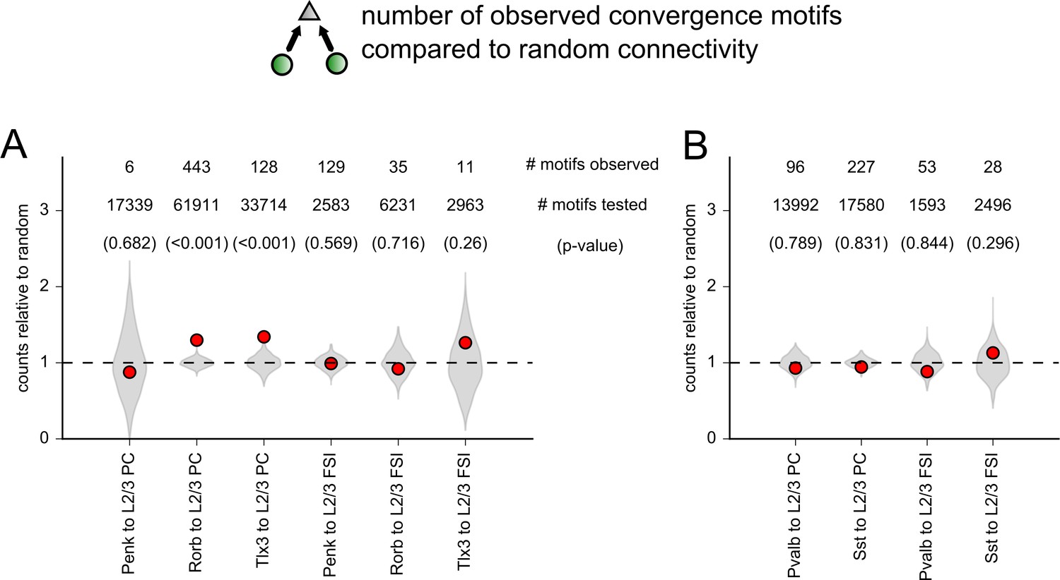
Comparison of the number of observed convergence motifs to a random network.
(A) Abundance of convergence motifs (two presynaptic cells to one postsynaptic cell) observed in data from each excitatory Cre line to either L2/3 pyramidal cells (PCs) or L2/3 fast-spiking interneurons (FSIs). Gray regions are violin plots of the distribution of convergence motifs observed in 1000 simulations of each dataset. Simulations were performed with experimentally measured distance dependence and postsynaptic subclass dependence (either L2/3 PCs or L2/3 FSIs) assigned to each tested connection. Red markers represent the number of convergence motifs observed in the experimental dataset. The distribution of simulations and observed values is each normalized to the average number of convergence motifs counted across all 1000 simulations. Numbers near the top of the plot indicate the number of motifs observed, the number of potential motifs tested, and the p-value derived from the distribution of random simulations (in parentheses). (B) Same as panel (A) for inhibitory Cre lines.
Figure 9—figure supplement 2
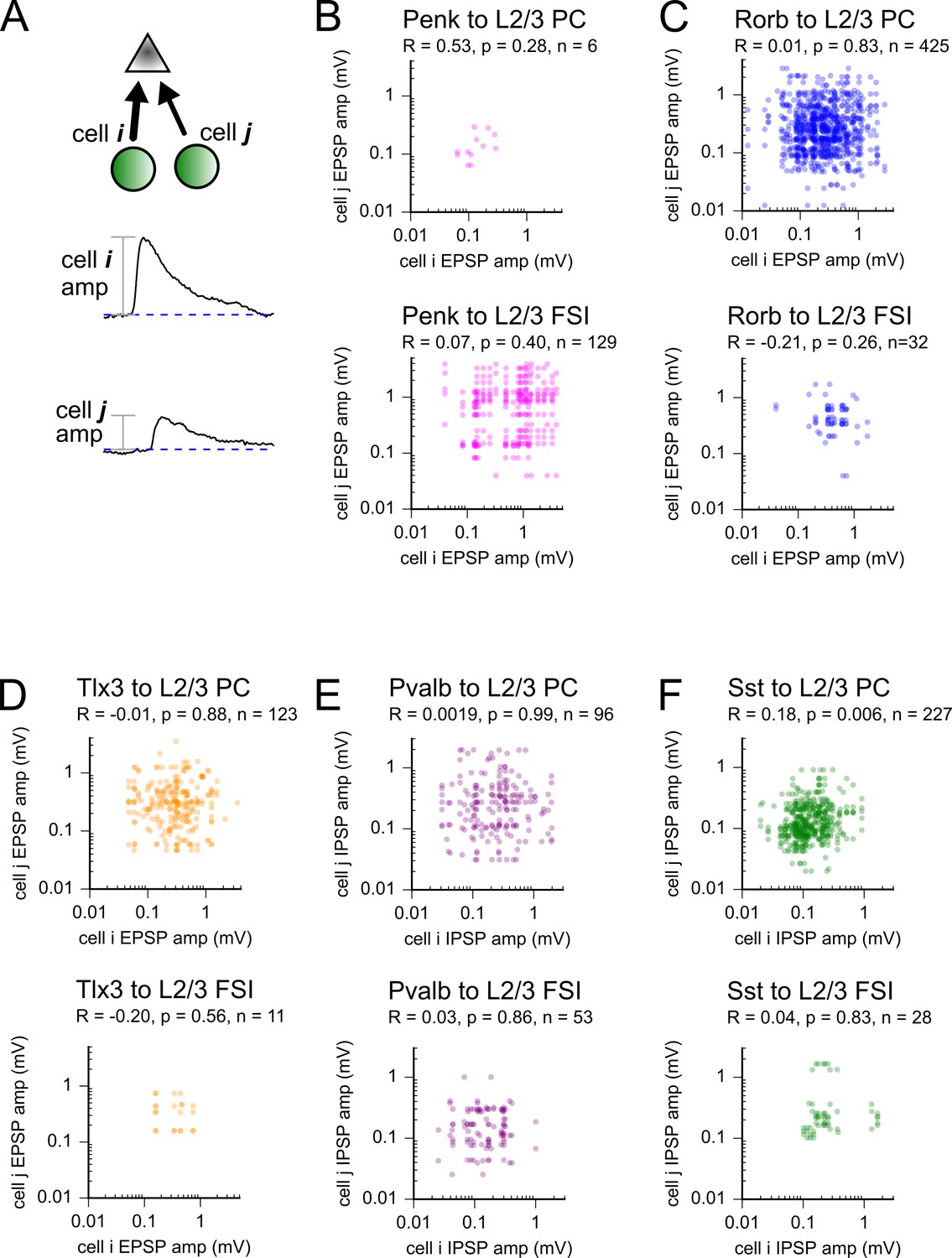
Scatter plots of incoming connections strengths for all pairs of cells sharing a postsynaptic partner for each Cre line and postsynaptic cell class.
(A) Cartoon of converging connections and amplitude measurements. (B–F) Scatter plots of incoming connection strength for all pairs of photostimulated cells sharing a postsynaptic partner. Data are split according to presynaptic Cre line and postsynaptic target (see labels above each plot). Strength of correlations (Pearson’s R measured in log-space), p-values, and number of unique pairs are reported under each heading.
Figure 10 with 1 supplement
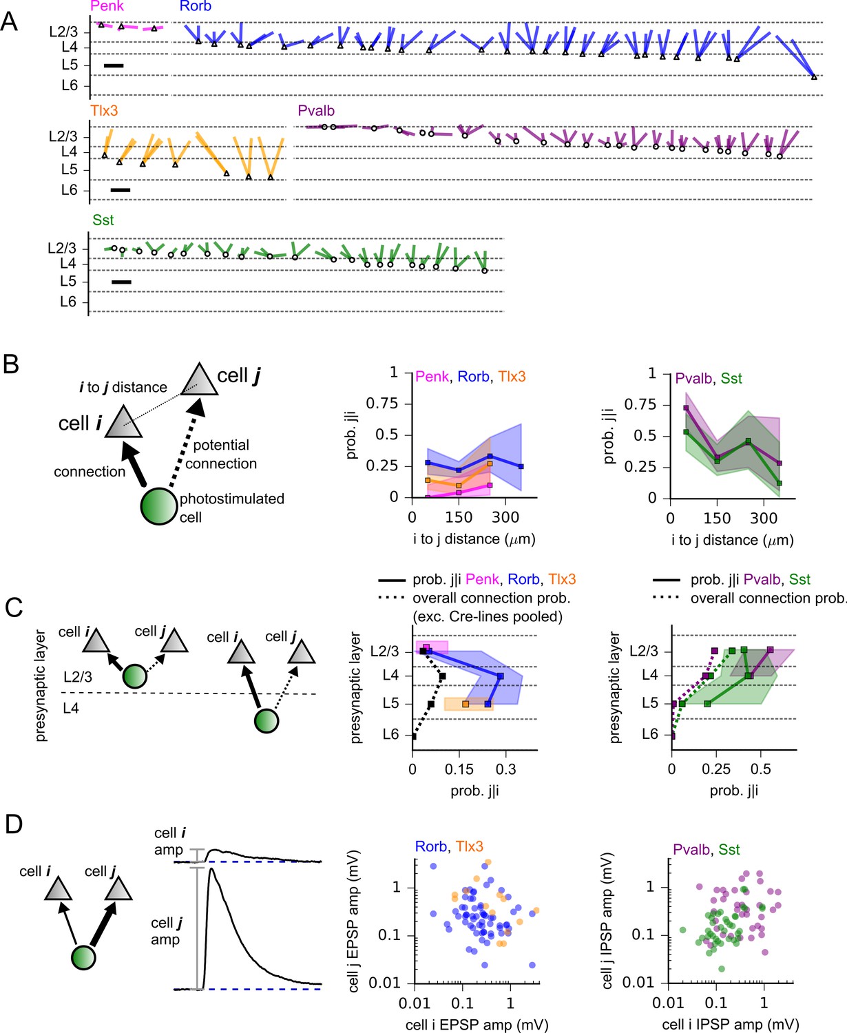
Divergence of synaptic outputs.
(A) All identified instances of divergent output to multiple neurons in L2/3 from Penk (magenta), Rorb (blue), Tlx3 (orange), Pvalb (purple), and Sst (green)-labeled presynaptic cells. The same colors are used to indicate Cre lines throughout the figure. Lines are drawn from presynaptic neurons (noted by triangles and circles for excitatory and inhibitory Cre lines, respectively) to 2–4 points representing the recipient cells. Cases of divergence are ordered according to the distance of the presynaptic cell from the pia. Scale bars = 200 µm. (B, left) Cartoon of completed divergence measurement. We first considered all unique ordered pairs of patch-clamped postsynaptic neurons (gray) that shared a possible presynaptic cell assayed by photostimulation (green). We then subset the data for all pairs in which the first cell (cell i) received a connection from the presynaptic cell (bold arrow). From this subset, we measured the fraction of pairs in which the second postsynaptic cell (cell j) also received a connection from the photostimulated cell. Middle: The probability of completed divergence (prob. j|i) plotted against the total intersomatic distance (Euclidean distance in three dimensions) between postsynaptic cells for excitatory Cre lines. Experiments performed using Penk or Tlx3 Cre lines did not include recordings of postsynaptic cells separated by more than 300 µm. Right: same as the middle panel for inhibitory Cre lines. (C) Prob. j|i was calculated as in panel (B), except data were grouped by the cortical layer of the presynaptic neuron. Dotted lines in the middle and right panels represent total connection probabilities measured across all tested connections to L2/3 pyramidal cells (PCs). To facilitate comparison between divergence and total connection probabilities, divergence was only calculated for pairs in which cell j was a L2/3 PC. Shading represents 95% confidence intervals. (D) Scatter plots of outgoing connection strengths for all pairs of L2/3 PCs sharing a presynaptic partner for each Cre line.
-
Figure 10—source data 1
Raw values for plots in Figure 10.
- https://cdn.elifesciences.org/articles/71103/elife-71103-fig10-data1-v2.xlsx
Figure 10—figure supplement 1
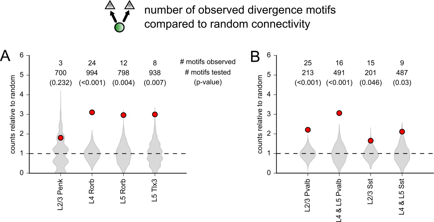
Comparison of the number of observed divergence motifs to a random network.
(A) Abundance of divergence motifs (one presynaptic cell to two postsynaptic cells) observed compared to a random network for each excitatory Cre line. Rorb cells were split by cortical layer. Gray violin plots represent the distribution of the number divergence motifs observed in 1000 simulations of each dataset. Simulations were performed with experimentally measured distance dependence and postsynaptic subclass dependence assigned to each tested connection. Red markers represent the number of divergence motifs observed in the experimental datasets. The distribution of simulations and observed values is each normalized to the average number of divergence motifs counted across all 1000 simulations. Numbers at the top of the plot indicate the number of divergence motifs observed, the number of divergence motifs tested in each dataset, and the p-value derived from the distribution of random simulations (in parentheses). (B) Same as panel (A) for inhibitory Cre lines split into intralaminar (L2/3) and translaminar (L4 and L5) groups.
Tables
Table 1
Comparison of synaptic connectivity measured by two-photon optogenetics to paired recordings.
Distance refers to Euclidean distance measured in three dimensions. Fisher’s exact p-values are reported before correcting for multiple comparisons. Benjamini–Hochberg p-values were calculated from Fisher’s exact p-values with a false discovery rate set to 0.25.
| Connection class | Distance (μm) | Paired recording connections (found/probed) | 2P opto connections (found/probed) | Paired recording connection probability | 2P opto connection probability | Fisher’s exact p-value | Benjamini–Hochberg p-value |
|---|---|---|---|---|---|---|---|
| Exc. to exc. | 0–100 | 8/135 | 12/205 | 0.06 | 0.06 | 1 | 1 |
| 100–200 | 2/48 | 3/312 | 0.04 | 0.01 | 0.13 | 0.51 | |
| Exc. to Pvalb | 0–100 | 13/28 | 19/41 | 0.46 | 0.46 | 1 | 1 |
| 100–200 | 8/27 | 9/60 | 0.3 | 0.15 | 0.15 | 0.51 | |
| Exc. to VIP | 0–100 | 6/25 | 7/24 | 0.24 | 0.29 | 0.75 | 1 |
| 100–200 | 4/28 | 0/11 | 0.14 | 0 | 0.31 | 0.72 | |
| Sst to exc. | 0–100 | 9/38 | 45/101 | 0.24 | 0.45 | 0.03 | 0.44 |
| 100–200 | 6/22 | 38/167 | 0.27 | 0.23 | 0.6 | 1 | |
| Sst to Pvalb | 0–100 | 8/36 | 2/12 | 0.22 | 0.17 | 1 | 1 |
| 100–200 | 4/35 | 4/26 | 0.11 | 0.15 | 0.71 | 1 | |
| Pvalb to exc. | 0–100 | 17/31 | 17/50 | 0.55 | 0.34 | 0.1 | 0.51 |
| 100–200 | 9/30 | 18/96 | 0.3 | 0.19 | 0.21 | 0.58 | |
| Pvalb to Pvalb | 0–100 | 30/82 | 6/17 | 0.37 | 0.35 | 1 | 1 |
| 100–200 | 32/102 | 14/35 | 0.31 | 0.4 | 0.41 | 0.82 |
Table 2
Properties of two-photon-evoked PSPs.
| Connection class | Amp. mean (mV) | Amp. median (mV) | Amp. sd (mV) | Amp. skew | n | CV | 20–80% rise (ms) |
|---|---|---|---|---|---|---|---|
| Penk to L2/3 PC | 0.17 | 0.15 | 0.1 | 1.3 | 16 | 0.8 | 1.92 |
| Rorb to L2/3 PC | 0.38 | 0.25 | 0.42 | 3.02 | 245 | 0.63 | 2.01 |
| Tlx3 to L2/3 PC | 0.46 | 0.30 | 0.51 | 3.2 | 85 | 0.54 | 1.72 |
| Ntsr1 to L2/3 PC | 0.09 | 0.09 | 1 | 1.09 | 1.19 | ||
| Penk to L2/3 FSI | 1.00 | 0.81 | 0.99 | 1.41 | 28 | 0.9 | 1.52 |
| Rorb to L2/3 FSI | 0.55 | 0.40 | 0.38 | 1.3 | 24 | 0.75 | 1.23 |
| Tlx3 to L2/3 FSI | 0.4 | 0.44 | 0.22 | 0.18 | 9 | 0.75 | 1.16 |
| Pvalb to L2/3 PC | 0.41 | 0.27 | 0.45 | 1.97 | 77 | 0.58 | 3.04 |
| Sst to L2/3 PC | 0.16 | 0.11 | 0.13 | 2.35 | 162 | 0.85 | 4.51 |
| Pvalb to L2/3 FSI | 0.21 | 0.16 | 0.18 | 2.61 | 34 | 0.86 | 2.03 |
| Sst to L2/3 FSI | 0.34 | 0.19 | 0.42 | 2.38 | 18 | 0.75 | 2.73 |
-
PSP: postsynaptic potential; PC: pyramidal cell; FSI: fast-spiking interneuron.
Table 3
Distance dependence of EPSP and IPSP amplitudes.
The strength and significance of correlations between PSP amplitudes and horizontal distance or the presynaptic neuron’s distance from the pia. Benjamini–Hochberg (BH)-corrected p-values were calculated using a false discovery rate of 0.1.
| Connection class | Horizontal Spearman’s R | Horizontal Spearman’s p-value | Horizontal BH-corrected p-value | Presyn. pia Spearman’s R | Presyn. pia Spearman’s p-value | Presyn. pia BH-corrected p-value | n |
|---|---|---|---|---|---|---|---|
| Penk to L2/3 PC | –0.53 | 0.04 | 0.12 | –0.51 | 0.05 | 0.23 | 16 |
| Rorb to L2/3 PC | 0.08 | 0.21 | 0.27 | 0.03 | 0.65 | 0.90 | 244 |
| Tlx3 to L2/3 PC | 0.18 | 0.09 | 0.17 | –0.01 | 0.91 | 0.91 | 85 |
| Penk to L2/3 FSI | –0.35 | 0.07 | 0.17 | –0.44 | 0.02 | 0.18 | 28 |
| Rorb to L2/3 FSI | –0.27 | 0.19 | 0.27 | –0.05 | 0.80 | 0.90 | 24 |
| Tlx3 to L2/3 FSI | 0.72 | 0.03 | 0.12 | 0.57 | 0.11 | 0.35 | 9 |
| Pvalb to L2/3 PC | 0.08 | 0.51 | 0.57 | 0.17 | 0.14 | 0.35 | 77 |
| Sst to L2/3 PC | 0.19 | 0.02 | 0.12 | 0.04 | 0.58 | 0.90 | 162 |
| Pvalb to L2/3 FSI | –0.07 | 0.68 | 0.68 | 0.04 | 0.81 | 0.90 | 34 |
| Sst to L2/3 FSI | 0.40 | 0.10 | 0.17 | 0.13 | 0.62 | 0.90 | 18 |
-
PSP: postsynaptic potential; PC: pyramidal cell; FSI: fast-spiking interneuron.
Key resources table
| Reagent type (species) or resource | Designation | Source or reference | Identifiers | Additional information |
|---|---|---|---|---|
| Genetic reagent (Mus musculus) | B6.FVB(Cg)-Tg(Ntsr1-cre)GN220Gsat/Mmucd | MMRRC | RRID:MMRRC_030648-UCD | |
| Genetic reagent (M. musculus) | B6;129S-Penktm2(cre)Hze/J | The Jackson Laboratory | RRID:IMSR_JAX:025112 | |
| Genetic reagent (M. musculus) | B6;129P2-Pvalbtm1(cre)Arbr/J | The Jackson Laboratory | RRID:IMSR_JAX:008069 | |
| Genetic reagent (M. musculus) | B6;129S-Rorbtm1.1(cre)Hze/J | The Jackson Laboratory | RRID:IMSR_JAX:023526 | |
| Genetic reagent (M. musculus) | B6;C3-Tg(Scnn1a-cre)3Aibs/J | The Jackson Laboratory | RRID:IMSR_JAX:009613 | |
| Genetic reagent (M. musculus) | B6J.Cg-Ssttm2.1(cre)Zjh/MwarJ | The Jackson Laboratory | RRID:IMSR_JAX:028864 | |
| Genetic reagent (M. musculus) | B6.FVB(Cg)-Tg(Tlx3-cre)PL56Gsat/Mmucd | MMRRC | RRID:MMRRC_041158-UCD | |
| Genetic reagent (M. musculus) | Ai167(TIT2L-ChrimsonR-tdT-ICL-tTA2) | Available from Allen Institute | ||
| RecombinantDNA reagent | flex-ChrimsonR-EYFP-Kv | Addgene | RRID:Addgene_135319 | |
| Software, algorithm | ACQ4 | http://www.acq4.org/, Campagnola et al., 2014 | RRID:SCR_016444, | |
| Software, algorithm | Igor Pro | WaveMetrics | RRID:SCR_000325 | |
| Software, algorithm | MIES: Software for Electrophysiology functions | Allen Institute | RRID:SCR_016443 |
Table 4
Intrinsic physiological properties of recorded neurons.
Measured intrinsic values for L2/3 PCs and L2/3 interneurons. Data are presented as mean ± SD.
| Cell class | L2/3 PC | L2/3 FSI | L2/3 VIP | L2/3 Sst |
|---|---|---|---|---|
| Vrest (mV) | –72.8 ± 6.7 | –68.2 ± 7.3 | –62.6 ± 10.5 | –61.8 ± 4.6 |
| Input resistance (MΩ) | 90.3 ± 31.5 | 92.4 ± 33.8 | 174 ± 64.3 | 199 ± 57.0 |
| Tau (ms) | 14.4 ± 4.3 | 6.5 ± 1.8 | 9.9 ± 4.3 | 16.8 ± 4.3 |
| Capacitance (pF) | 171 ± 58 | 80 ± 44 | 56 ± 15 | 87 ± 20 |
| Sag | 0.032 ± 0.027 | 0.062 ± 0.042 | 0.117 ± 0.068 | 0.16 ± 0.096 |
| Rheobase (pA) | 171 ± 75 | 268 ± 119 | 126 ± 77 | 129 ± 52 |
| FWHM (ms) | 1.37 ± 0.31 | 0.62 ± 0.17 | 1.25 ± 0.29 | 0.79 ± 0.14 |
| Upstroke-downstroke ratio | 4.30 ± 0.68 | 1.72 ± 0.23 | 3.36 ± 0.58 | 2.10 ± 0.36 |
| AP peak (mV) | 40.6 ± 8.0 | 19.5 ± 7.9 | 27.5 ± 12.7 | 24.0 ± 13.4 |
| AP trough (mV) | –48.4 ± 4.9 | –53.0 ± 5.16 | –51.0 ± 2.8 | –52.7 ± 5.2 |
| AP height (mV) | 89.0 ± 10.1 | 72.5 ± 10.2 | 78.5 ± 13.1 | 76.7 ± 17.0 |
| Average firing rate (spikes/s) | 7.78 ± 2.36 | 30.9 ± 10.8 | 15.5 ± 11.3 | 15.6 ± 6.6 |
| Adaptation | 0.090 ± 0.079 | 0.008 ± 0.021 | 0.044 ± 0.083 | 0.081 ± 0.090 |
| f-i slope (spikes/s/pA) | 0.12 ± 0.06 | 0.66 ± 0.19 | 0.20 ± 0.11 | 0.29 ± 0.11 |
-
PC: pyramidal cell; AP: action potential; FWHM: full-width at half-maximum.
Table 5
Features measured for all photostimulus responses.
| Features from average response | Features from deconvolved average response | Features from individual deconvolved responses |
|---|---|---|
| Maximum amplitude of response (peak) | Peak of deconvolved average (deconvolved peak) | Average number of times each trace exceeded 3× deconvolved SD |
| Time of peak | Time of deconvolved peak | SD of number of crossings per sweep |
| Standard deviation (SD) at time of peak | SD of deconvolved trace in baseline window (deconvolved SD) | |
| SD in baseline window | Number of times the deconvolved trace exceeded 3× deconvolved SD | |
| Number of times the deconvolved trace exceeded 5× deconvolved SD |
Author response table 1
| I-clamp connected /probed | V-clamp connected /probed | I-clamp connection probability | V-clamp connection probability | Fisher's Exact pvalue (I-clamp vs V-clamp) | Fisher’s Exact odds ratio | |
|---|---|---|---|---|---|---|
| L2/3 Sst:Ai167 to L2/3 pyr. cell | 24/52 | 16/25 | 0.46 | 0.64 | 0.15 | 0.48 |
| Translaminar(L4/L5)Sst:Ai167 toL2/3 pyr. cell | 2/71 | 6/73 | 0.03 | 0.08 | 0.28 | 0.32 |
| L5 Sst:Ai167 to L5 pyr. cell | 25/147 | 20/68 | 0.17 | 0.29 | 0.05 | 0.49 |
Additional files
Download links
A two-part list of links to download the article, or parts of the article, in various formats.
Downloads (link to download the article as PDF)
Open citations (links to open the citations from this article in various online reference manager services)
Cite this article (links to download the citations from this article in formats compatible with various reference manager tools)
Synaptic connectivity to L2/3 of primary visual cortex measured by two-photon optogenetic stimulation
eLife 11:e71103.
https://doi.org/10.7554/eLife.71103


