Figures and data in Nonlinear transient amplification in recurrent neural networks with short-term plasticity

Figures
Tables
Additional files

6 figures, 15 tables and 1 additional file

Figures

Figure 1 with 1 supplement

Download asset Open asset

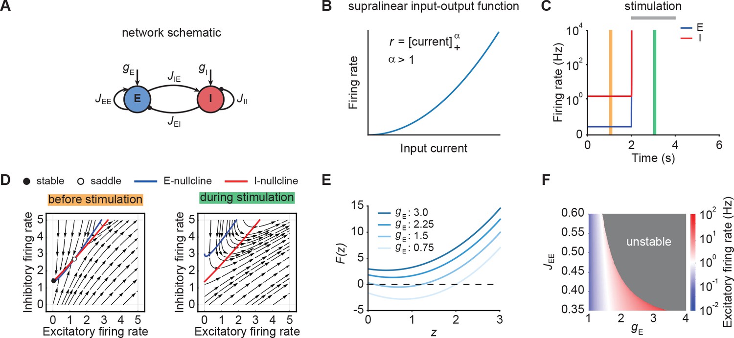
Neuronal ensembles nonlinearly amplify inputs above a critical threshold.

(A) Schematic of the recurrent ensemble model consisting of an excitatory (blue) and an inhibitory population (red). (B) Supralinear input-output function given by a rectified power law with exponent $α = 2$ . (C) Firing rates of the excitatory (blue) and inhibitory population (red) in response to external stimulation during the interval from 2 to 4 s (gray bar). The stimulation was implemented by temporarily increasing the input $g_{E}$ . (D) Phase portrait of the system before stimulation (left; C orange) and during stimulation (right; C green). (E) Characteristic function $F (z)$ for varying input strength $g_{E}$ . Note that the function loses its zero crossings, which correspond to fixed points of the system for increasing external input. (F) Heat map showing the evoked firing rate of the excitatory population for different parameter combinations $J_{E E}$ and $g_{E}$ . The gray region corresponds to the parameter regime with unstable dynamics.

Figure 1—figure supplement 1

Download asset Open asset

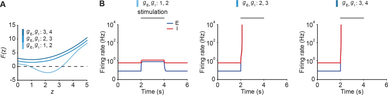
Unstable ensemble dynamics can be triggered by additional stimulation in supralinear networks with negative determinant even in the presence of substantial feedforward inhibition.

(A) Characteristic function $F (z)$ for different inputs $g_{E}$ and $g_{I}$ . (B) Firing rates of the excitatory (blue) and inhibitory population (red) in response to stimulation from 2 to 4 s (gray bar). During stimulation $g_{E}$ and $g_{I}$ are simultaneously changed to the stated values.

Figure 2 with 12 supplements

Download asset Open asset

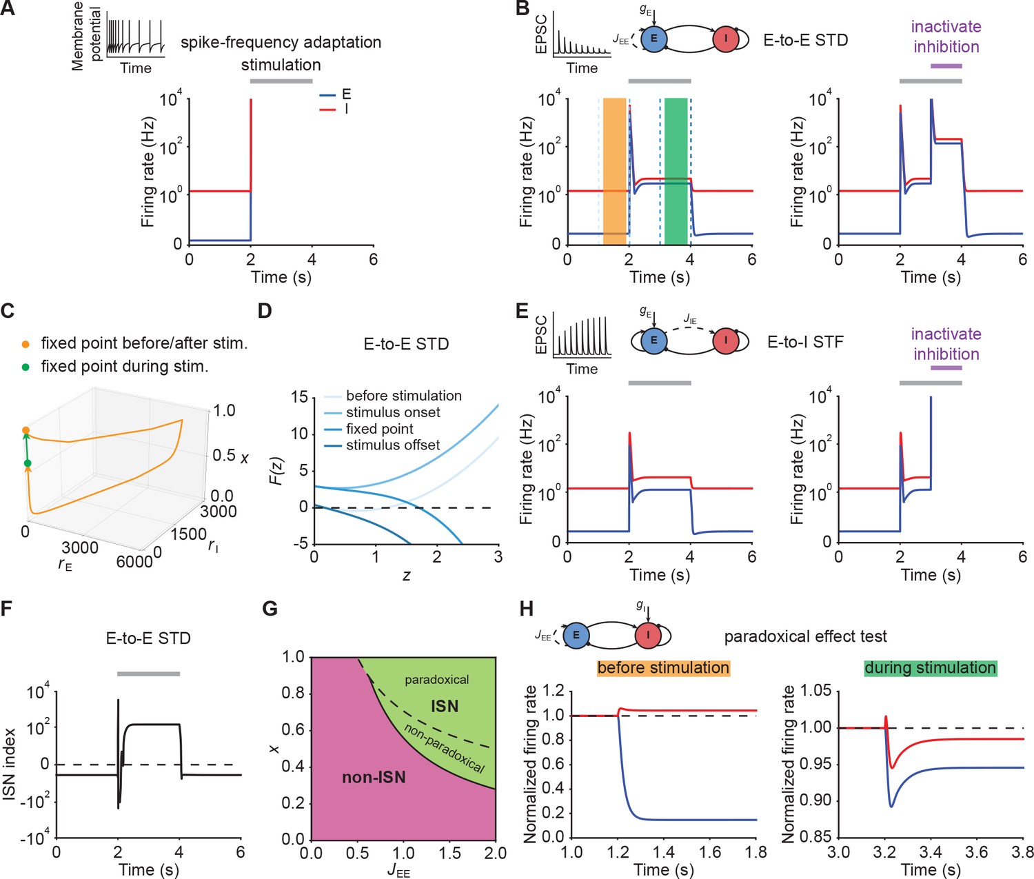
Short-term plasticity, but not spike-frequency adaptation, re-stabilizes ensemble dynamics.

(A) Firing rates of the excitatory (blue) and inhibitory population (red) in the presence of spike-frequency adaptation (SFA). During stimulation (gray bar) additional input is injected into the excitatory population. The inset shows a cartoon of how SFA affects spiking neuronal dynamics in response to a step current input. (B) Left: Same as (A) but in the presence of E-to-E short-term depression (STD). Right: Same as left but inactivating inhibition in the period marked in purple. (C) 3D plot of the excitatory activity $r_{E}$ , inhibitory activity $r_{I}$ , and the STD variable $x$ of the network in B left. The orange and green points mark the fixed points before/after and during stimulation. (D) Characteristic function $F (z)$ in networks with E-to-E STD. Different brightness levels correspond to different time points in B left. (E) Same as (B) but in the presence of E-to-I short-term facilitation (STF). (F) Inhibition-stabilized network (ISN) index, which corresponds to the largest real part of the eigenvalues of the Jacobian matrix of the E-E subnetwork with STD, as a function of time for the network with E-to-E STD in B left. For values above zero (dashed line), the ensemble is an ISN. (G) Analytical solution of non-ISN (magenta), ISN (green), paradoxical, and non-paradoxical regions for different parameter combinations $J_{E E}$ and the STD variable $x$ . The solid line separates the non-ISN and ISN regions, whereas the dashed line separates the non-paradoxical and paradoxical regions. (H) The normalized firing rates of the excitatory (blue) and inhibitory population (red) when injecting additional excitatory current into the inhibitory population before stimulation (left; orange bar in B), and during stimulation (right; green bar in B). Initially, the ensemble is in the non-ISN regime and injecting excitatory current into the inhibitory population increases its firing rate. During stimulation, however, the ensemble is an ISN. In this case, excitatory current injection into the inhibitory population results in a reduction of its firing rate, also known as the *paradoxical effect*.

Figure 2—figure supplement 1

Download asset Open asset

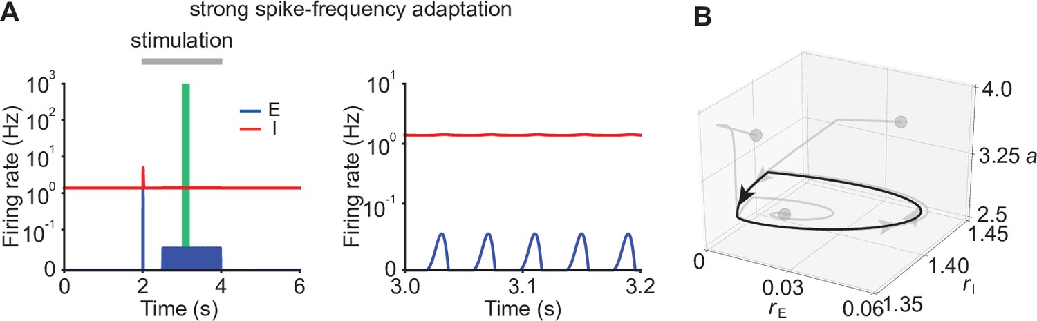
Ensemble dynamics in supralinear networks with strong SFA.

(A) Firing rates of the excitatory (blue) and inhibitory population (red) in the presence of strong SFA (left) with $b = 200$ . The zoomed-in activity from 3.0 s to 3.2 s (right) corresponding to the green period (left) indicates oscillatory behavior in networks with strong SFA. (B) 3D plot of the excitatory activity $r_{E}$ , inhibitory activity $r_{I}$ , and the SFA variable $a$ of the network in the period marked with the green bar in A. Networks with different conditions starting from different gray dots converge to the same stable limit cycle marked with the black line.

Figure 2—figure supplement 2

Download asset Open asset

Dependence of peak amplitude and fixed point activity on input g_E and E-to-E connection strength J_EE.

(A) The onset peak amplitude (triangles) and fixed point activity (circles) as a function of input $g_{E}$ in networks with E-to-E STD. Here, $J_{E E} = 1.8$ . (B) The ratio of the onset peak amplitude to fixed point activity as a function of input $g_{E}$ . The vectical dashed line indicates the input level which leads to unstable network dynamics without E-to-E STD. (**C and D**) Same as A and B but as a function of $J_{E E}$ . Here, $g_{E} = 2.0$ .

Figure 2—figure supplement 3

Download asset Open asset

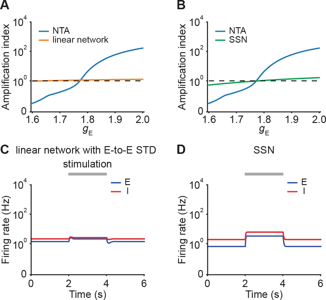
Comparisons of amplification ability between NTA and linear networks, and between NTA and SSNs.

(A) Amplification index,which is defined as the ratio of the peak amplitude to input $g_{E}$ , as a function of input $g_{E}$ for NTA (blue) and linear network (orange) in the presence of E-to-E STD. (B) Same as A but for SSN without STP (green).SSN is constructed by keep-ing $J_{E E}$ the same while changing $J_{I E}$ to $J_{I I}$ such that the determinant of the weight matrix det(J) becomes positive. (C) Example of firing rates of the excitatory (blue) and inhibitory population (red) in linear networks with E-to-E STD. During stimulation (gray bar) additional input is injected into the excitatory population. Same as Figure 2B (left) but with $α_{E} = α_{1} = 1$ and $g_{E} = 2$ . (D) Example of firing rates of the excitatory (blue) and inhibitory population (red) in SSNs with $g_{E} = 2$ .

Figure 2—figure supplement 4

Download asset Open asset

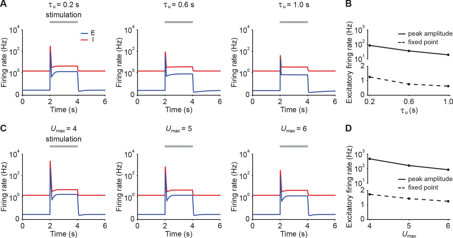
Dependence of peak amplitude and fixed point activity on STP parameters.

(A) Firing rates of the excitatory (blue) and inhibitory population (red) in response to stimulation in the presence of E-to-I STF with different time constants $τ_{u}$ . The stimulation period from 2 s to 4 s is marked with the gray bar. The stimulation is implemented by changing input $g E$ . (B) Peak amplitude (solid line) and fixed point activity (dashed line) of the excitatory population during stimulation with different STF time constants. (**C and D**) Same as A and B, but with different maximum allowed facilitation levels $U_{m a x}$ .

Figure 2—figure supplement 5

Download asset Open asset

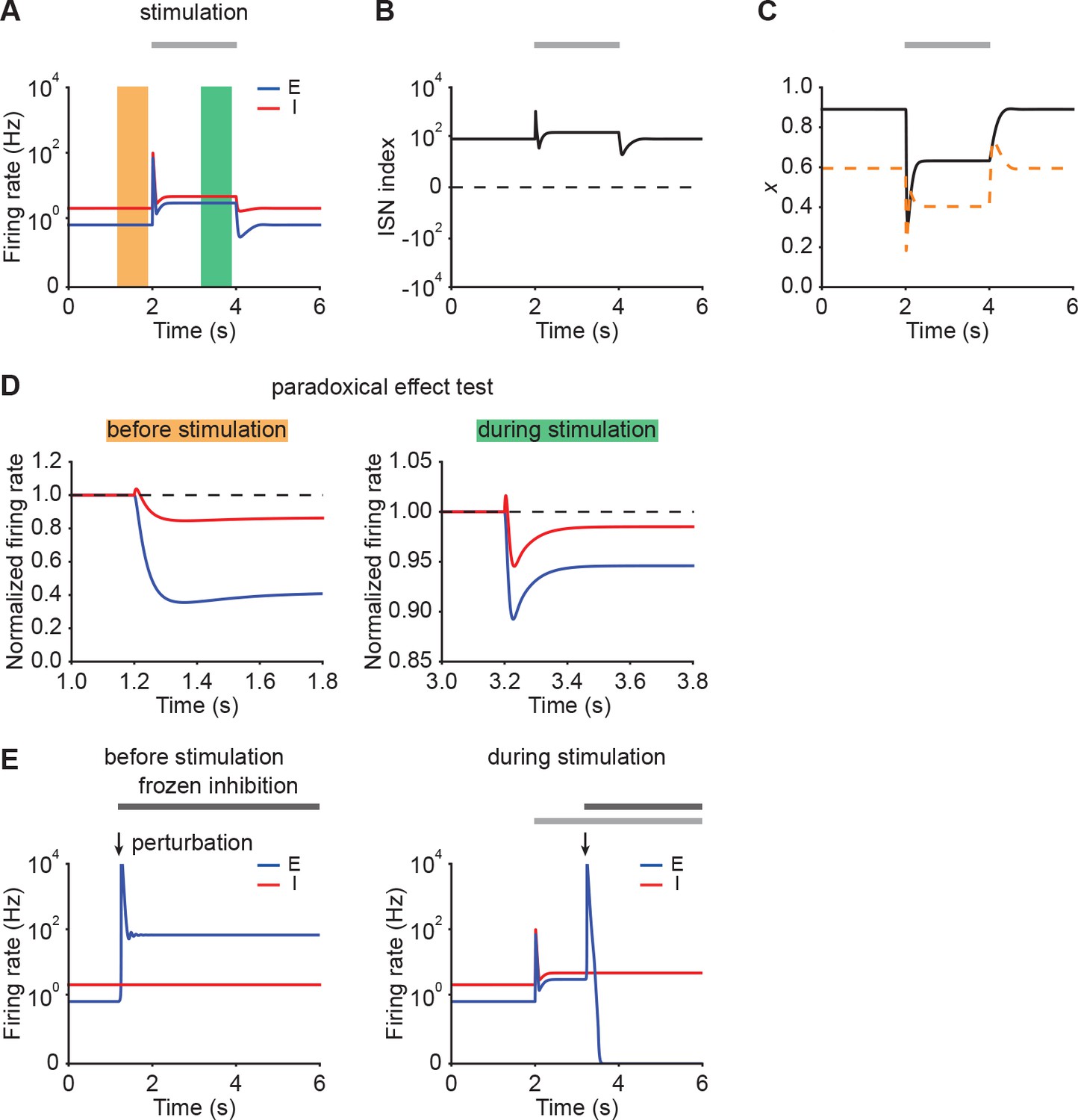
Networks initially in the ISN regime can exhibit strong NTA.

(A) Firing rates of the excitatory (blue) and inhibitory population (red) in the presence of E-to-E STD in an example of a network initially in the ISN regime. During stimulation (gray bar) additional input is injected into the excitatory population. (B) ISN index of the network. (C) Depression variable (black) in an example of a network shown in A. The orange dashed line represents the depression variable threshold above which the network exhibits the paradoxical effect. (D) The normalized firing rates of the excitatory (blue) and inhibitory population (red) when injecting additional excitatory current into the inhibitory population before stimulation (left; orange bar in A), and during stimulation (right; green bar in A). Both before stimulation and during stimulation, the ensemble is in the ISN regime and injecting excitatory current into inhibitory population decreases its firing rate. (E) Firing rates of the excitatory (blue) and inhibitory population (red) when a small transient perturbation to excitatory population activity is introduced marked with arrows while freezing inhibition before stimulation (left) and during stimulation (right). The periods in which inhibition is frozen are marked with black bars. Both before stimulation and during stimulation, the ensemble is in the ISN regime and a small transient excitatory perturbation to the excitatory population results in a transient explosion of the excitatory firing rate.

Figure 2—figure supplement 6

Download asset Open asset

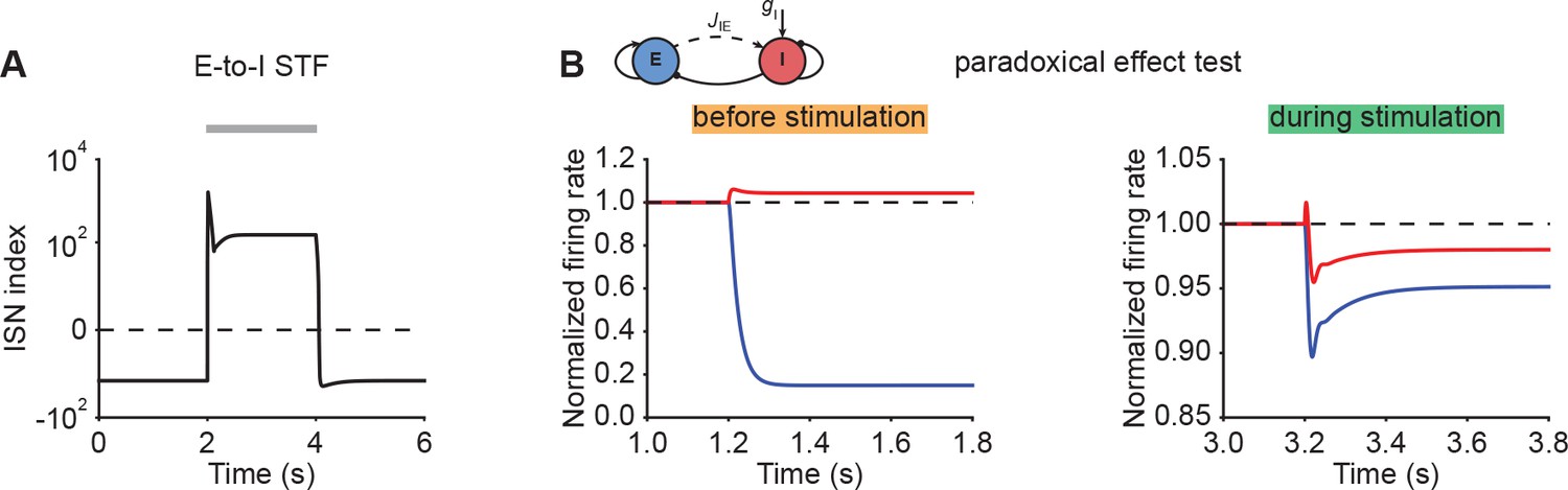
ISN index and paradoxical effect test for networks with E-to-I STF.

(A) ISN index of the network with E-to-I STF in Figure 2E (left). The horizontal dashed line indicates an ISN index of 0. (B) The normalized firing rates of the excitatory (blue) and inhibitory population (red) when injecting additional excitatory current into the inhibitory population before stimulation (left, Figure 2E), and during stimulation (right, Figure 2E). The horizontal dashed lines indicate a normalized firing rate of 1.0.

Figure 2—figure supplement 7

Download asset Open asset

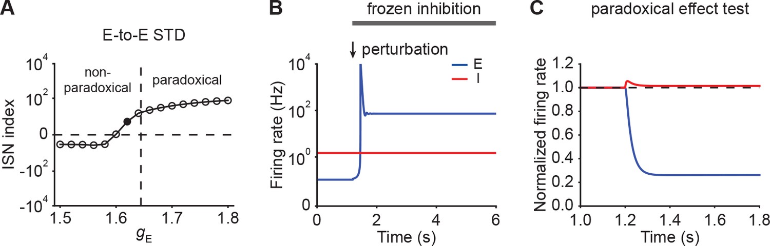
Inhibition stabilization does not imply paradoxical response in networks with E-to-E STD.

(A) ISN index of the network with E-to-E STD as a function of input $g_{E}$ . The horizontal dashed line indicates an ISN index of 0. For values above zero, the ensemble is an ISN. The vertical dashed line separates the non-paradoxical and paradoxical regions. (B) Firing rates of the excitatory (blue) and inhibitory population (red) in an ensemble with the input level marked with the black dot in A when a small transient perturbation to excitatory population activity is introduced marked with arrows while freezing inhibition. The periods in which inhibition is frozen are marked with the black bar. A small transient perturbation to the excitatory population results in a transient explosion of the excitatory firing rate, indicating that the ensemble is an ISN. (C) The normalized firing rates of the excitatory (blue) and inhibitory population (red) when injecting excitatory input into the inhibitory population of an ensemble with the input level marked with the black dot in A. The horizontal dashed line indicates a normalized firing rate of 1.0. Despite being an ISN, the ensemble does not exhibit the paradoxical effect.

Figure 2—figure supplement 8

Download asset Open asset

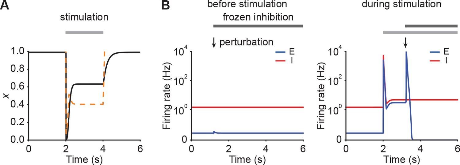
Transition from non-ISN to ISN indicating by frozen inhibition test.

(A) Depression variable (black) in an example of a network initially in the non-ISN regime shown in Figure 2B left. The orange dashed line represents the depression variable threshold above which the network exhibits the paradoxical effect. (B) Firing rates of the excitatory (blue) and inhibitory population (red) when a small transient perturbation to excitatory population activity is introduced marked with arrows while freezing inhibition before stimulation (left; Figure 2B left) and during stimulation (right; Figure 2B left). The periods in which inhibition is frozen are marked with black bars. Initially, the ensemble is in the non-ISN regime and the firing rate of the excitatory slightly increases and then returns to its baseline after introducing a small transient perturbation to the excitatory population. During stimulation, however, the ensemble is an ISN. In this case, a small transient perturbation to the excitatory population results in a transient explosion of the excitatory firing rate.

Figure 2—figure supplement 9

Download asset Open asset

Similar qualitative behavior in rate-based models with maximal firing rate capped at 300 Hz.

(A) Firing rates of the excitatory (blue) and inhibitory population (red) in response to stimulation in a rate-based model. Additional excitatory inputs are injected into excitatory neurons in the period marked in gray. Firing rates are capped at 300 Hz. (B) Same as A but incorporating SFA. (C) Same as A but incorporating E-to-E STD. (D) Same as A but incorporating E-to-I STF. (E) Same as B but incorporating stronger SFA (left). The zoomed-in activity from 3.0 s to 3.2 s (right) corresponding to the green period (left) indicates oscillatory behavior in networks with strong SFA.

Figure 2—figure supplement 10

Download asset Open asset

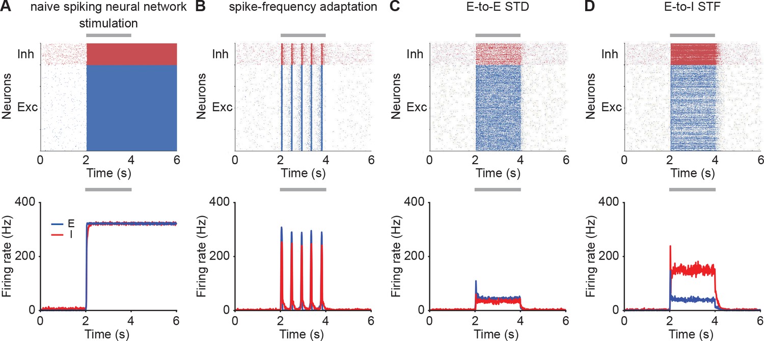
Similar qualitative behavior in spiking neural networks.

(A) Spike raster plot of the excitatory (top, blue) and inhibitory population (top, red) in response to stimulation in a spiking neural network model, and firing rates calculated with 10 ms time bins (bottom). Additional excitatory inputs are injected into excitatory neurons in the period marked in gray. (B) Same as A but incorporating SFA. (C) Same as A but incorporating E-to-E STD. (D) Same as A but incorporating E-to-I STF.

Figure 2—figure supplement 11

Download asset Open asset

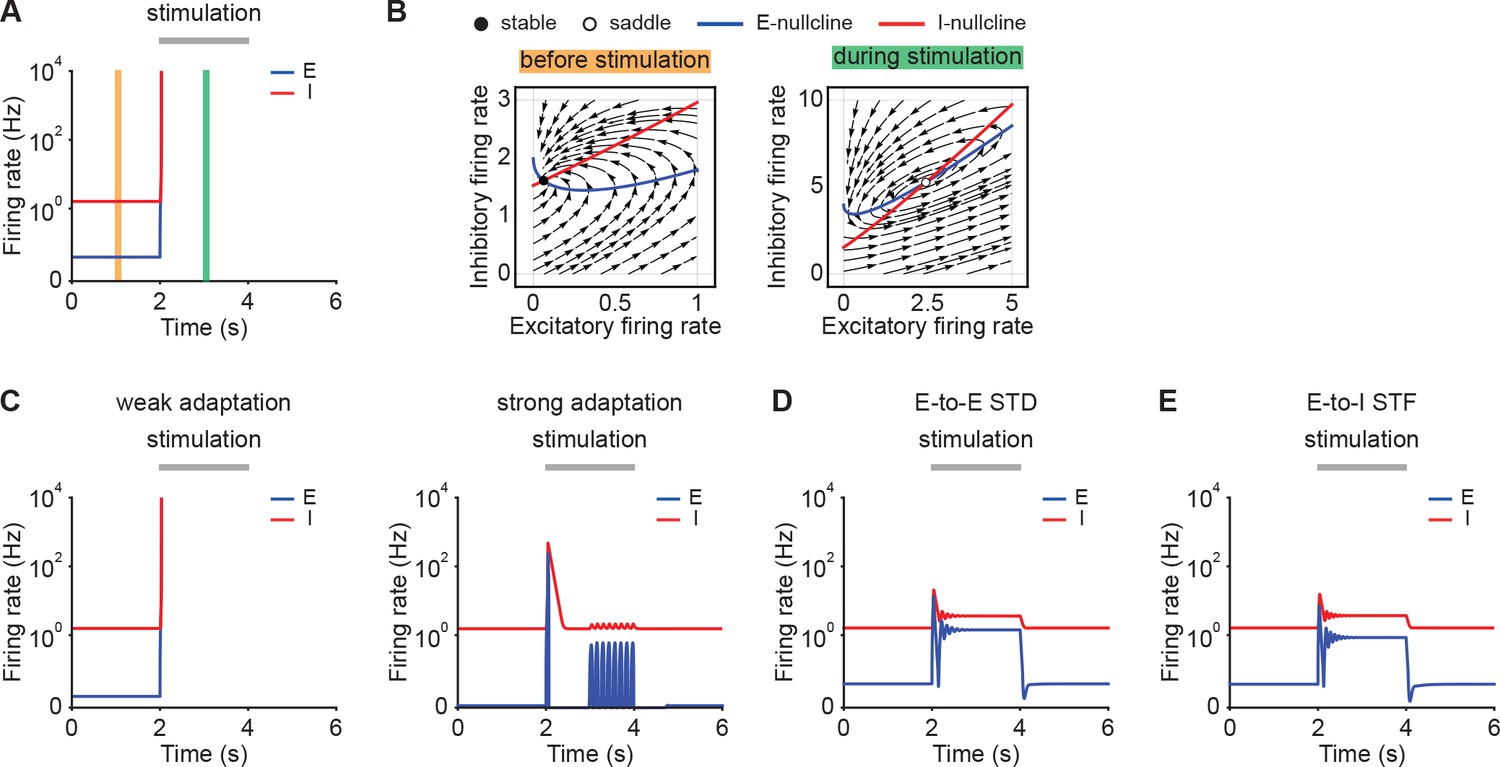
Unstable dynamics can emerge in supralinear networks with positive determinant and slow inhibition.

(A) Firing rates of the excitatory (blue) and inhibitory population (red) in networks with positive determinant in response to external stimulation during the interval from 2 to 4 s (gray bar). The stimulation was implemented by temporarily increasing the input $g_{E}$ . (B) Phase portrait of the system before stimulation (left; A orange) and during stimulation (right; A green). (C) Same as (A) but in the presence of weak SFA (left) and strong SFA (right). (D) Same as (A) but in the presence of E-to-E STD. (E) Same as (A) but in the presence of E-to-I STF.

Figure 2—figure supplement 12

Download asset Open asset

Networks with substantial feedforward inhibition can exhibit strong NTA.

(A) Example of activity when the change in the input of the inhibitory population Δg_t is larger than the the change in the input of the excitatory population Δg_E . Here, Δg_E = 1.8, and Δg_I = 3. (B) The ratio of the onset peak amplitude to the baseline activity as a function of the change in the input of the excitatory population Δg_E and the change in the input of the inhibitory population Δg_I . The diagonal dashed line indicates the border at which Δg_E is identical to Δg_I in networks with E-to-E STD. The star symbol represents the example shown in A.

Figure 3 with 1 supplement

Download asset Open asset

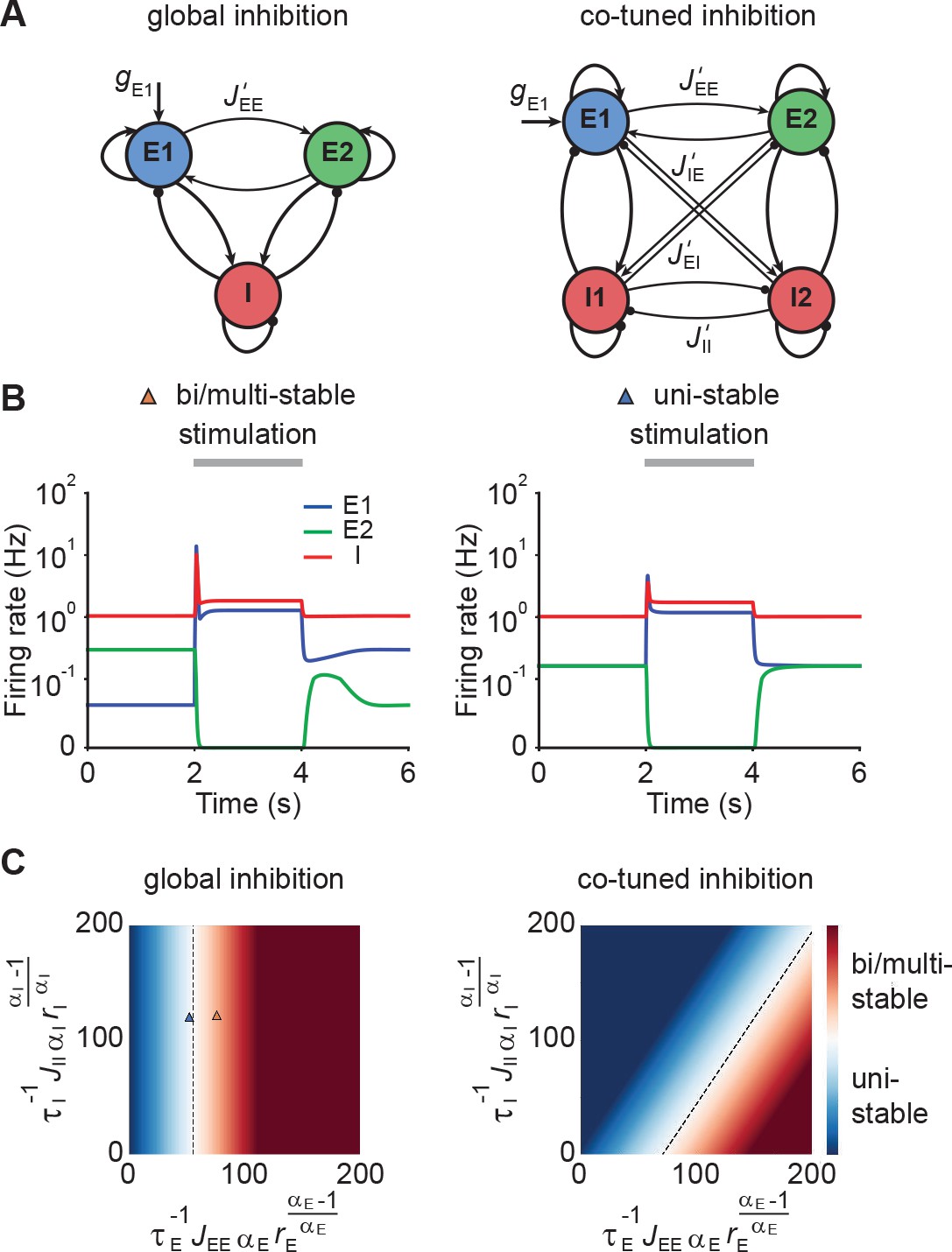
Co-tuned inhibition broadens the parameter regime of NTA in the absence of persistent activity.

(A) Schematic of two neuronal ensembles with global inhibition (left) and with co-tuned inhibition (right). (B) Firing rate dynamics of bi/multi-stable ensemble dynamics (left) and uni-stable (right). In both cases, additional excitatory inputs are injected into excitatory ensemble E1 during the period marked in gray. (C) Analytical solution of uni- and bi/multi-stability regions for global inhibition (left) and co-tuned inhibition (right). Co-tuning results in a larger parameter regime of uni-stability. The triangles correspond to the two examples in B.

Figure 3—figure supplement 1

Download asset Open asset

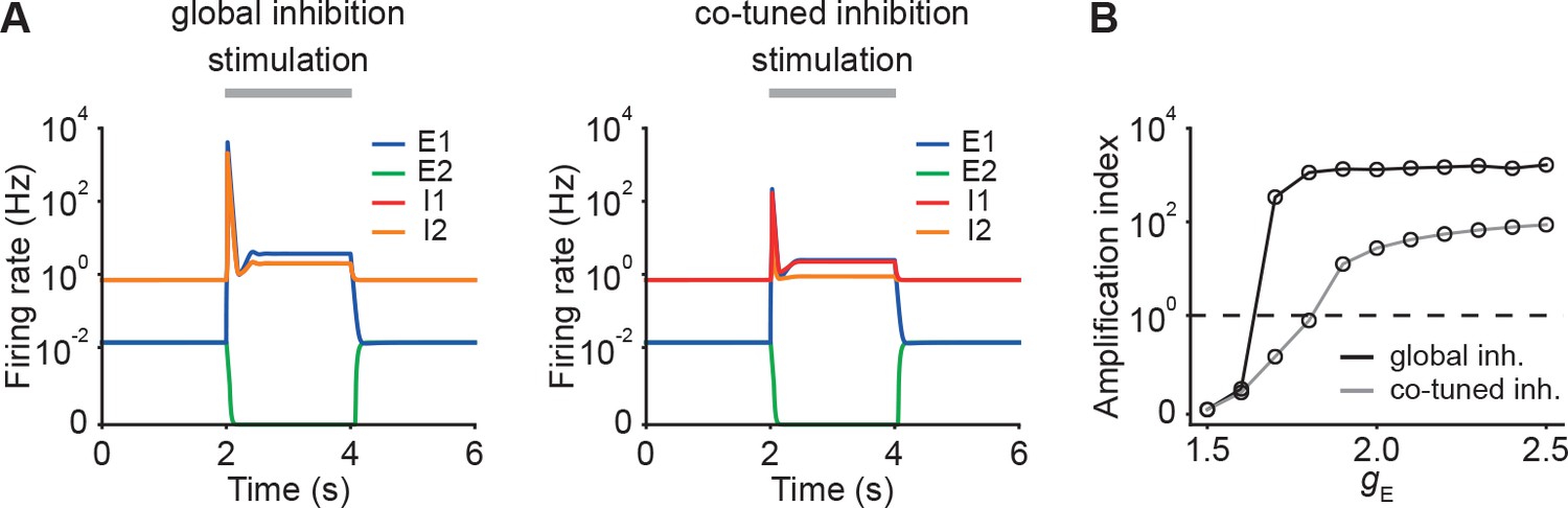
Ensembles with co-tuned inhibition exhibit weaker — but still strong — NTA in comparison to ensembles with global inhibition.

(A) Examples of activity in networks with global inhibition (left) and in networks with co-tuned inhibition (right) in the presence of E-to-E STD. (B) Amplification index for networks with global inhibition (black) and network with co-tuned inhibition (gray) as a function of input $g_{E}$ in networks with E-to-E STD. Data points at $g_{E} = 2.5$ correspond to the examples shown in A.

Figure 4 with 2 supplements

Download asset Open asset

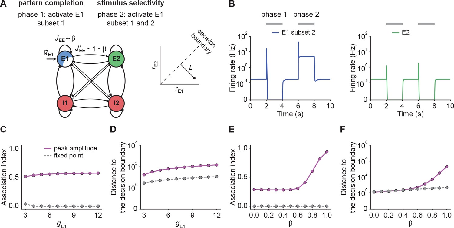
NTA yields stronger pattern completion than fixed points while retaining stimulus selectivity.

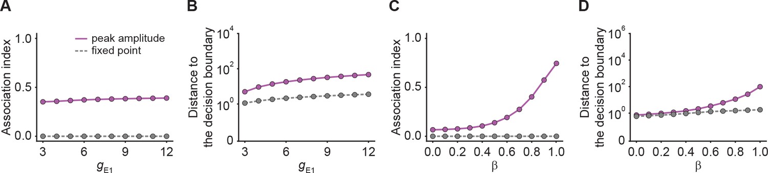
(A) Schematic of the network setup used to probe pattern completion and stimulus selectivity. To assess the effect on pattern completion, 75% of the neurons (Subset 1) in ensemble E1 received additional input g_E1 during Phase one (2–4 s), while we recorded the firing rate of the remaining 25% (Subset 2) in the excitatory ensemble E1. To evaluate the impact on stimulus selectivity, all neurons in E1 received additional inputs g_E1 in Phase two (6–8 s) while the firing rate of E2 was measured. A downstream neuron’s ability to discriminate between E1 or E2 being active depends on whether their activity is well separated by a symmetric decision boundary (inset). (B) Examples of firing rates of Subset 2 of E1 (left, blue) and E2 (right, green) with E-to-E STD. (C) Association index as a function of input g_E1 for the onset peak amplitude (magenta solid line) and fixed point activity (gray dashed line) for E-to-E STD. (D) Distance to the decision boundary (see panel A, inset) as a function of input g_E1 for the onset peak amplitude (magenta solid line) and fixed point activity (gray dashed line) for E-to-E STD. (**E and F**) Same as C and D but as a function of β, which controls the inner- and inter-ensemble connection strength.

Figure 4—figure supplement 1

Download asset Open asset

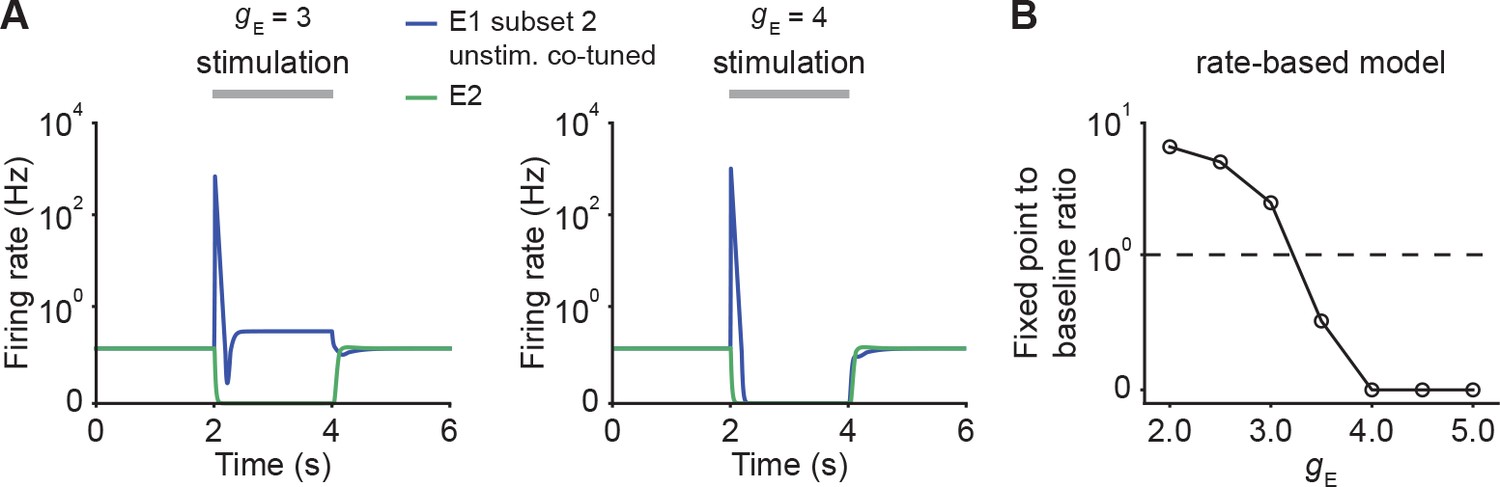
Change in steady state activity for unstimulated co-tuned neurons in the rate-based model.

(A) Examples of firing rates of Subset 2 of E1 (blue) and E2 (green) for g_E = 3 (left) and for g_E = 4 (right) in networks with E-to-E STD. (B) The ratio of the fixed point activity to the baseline activity for unstimulated co-tuned neurons (E1 Subset 2) as a function of input g_E in rate-based models with E-to-E STD. The horizontal dashed line indicates a ratio of 1 at which the fixed point activity is identical to the baseline activity.

Figure 4—figure supplement 2

Download asset Open asset

Quantification of pattern completion and stimulus selectivity in networks with E-to-I STF.

(A) Association index as a function of input g_E1 for the onset peak amplitude (magenta solid line) and fixed point activity (gray dashed line) for E-to-I STF. (B) Distance to the decision boundary as a function of input g_E1 for the onset peak amplitude (magenta solid line) and fixed point activity (gray dashed line) for E-to-I STF. (**C and D**) Same as A and B but as a function of β, which controls the inner- and inter-ensemble connection strength.

Figure 5 with 2 supplements

Download asset Open asset

NTA provides stronger amplification and pattern separation in morphing experiments than fixed point activity.

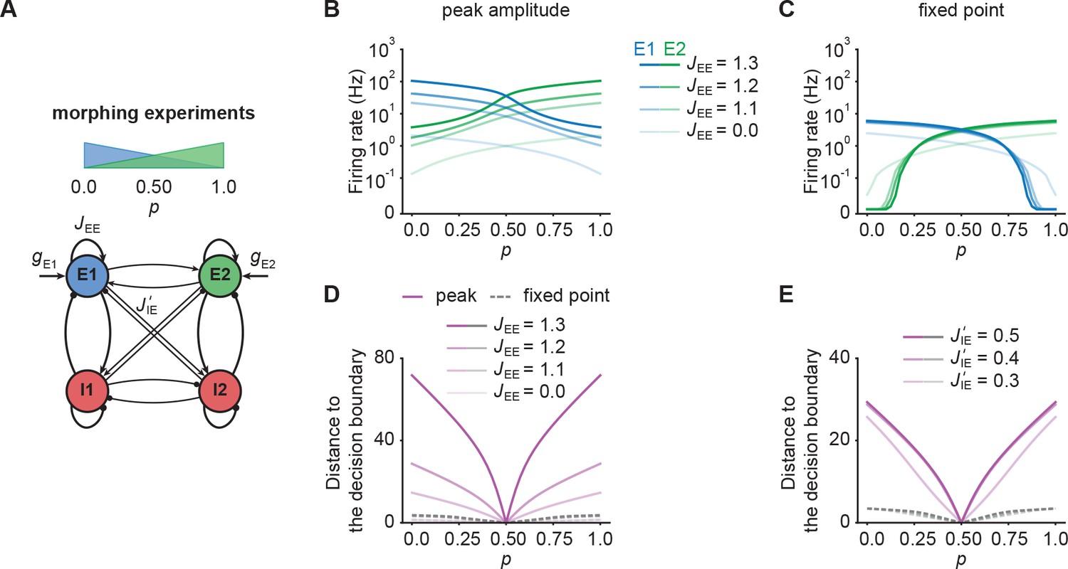
(A) Schematic of the morphing stimulation paradigm. The fraction of the additional inputs into the two excitatory ensembles is controlled by the parameter p. (B) Peak amplitude of E1 (blue) and E2 (green) as a function of p for E-to-E STD. Brightness levels represent different recurrent E-to-E connection strengths J_EE . (C) Same as in B but for fixed point activity. (D) Distance to the decision boundary as a function of p for the peak onset response (magenta solid line) and fixed point activity (gray dashed line) for E-to-E STD in a network with J’_IE = 0.4. (E) Same as D but with different E-to-I connection strengths J’_IE across ensembles for a network with J_EE = 1.2.

Figure 5—figure supplement 1

Download asset Open asset

Quantification of pattern separation in morphing experiments using a normalized measure.

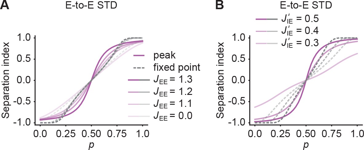
(A) Separation index, defined as $(r_{E 2} - r_{E 1}) / (r_{E 1} + r_{E 2})$ , as a function of p for the peak onset response (magenta solid line) and fixed point activity (gray dashed line) for E-to-E STD. Different levels of brightness represent different recurrent E-to-E connection strengths J_EE . (B) Same as A but with different E-to-I connection strengths J’_IE across ensembles.

Figure 5—figure supplement 2

Download asset Open asset

Quantification of pattern separation in morphing experiments for networks with E-to-I STF.

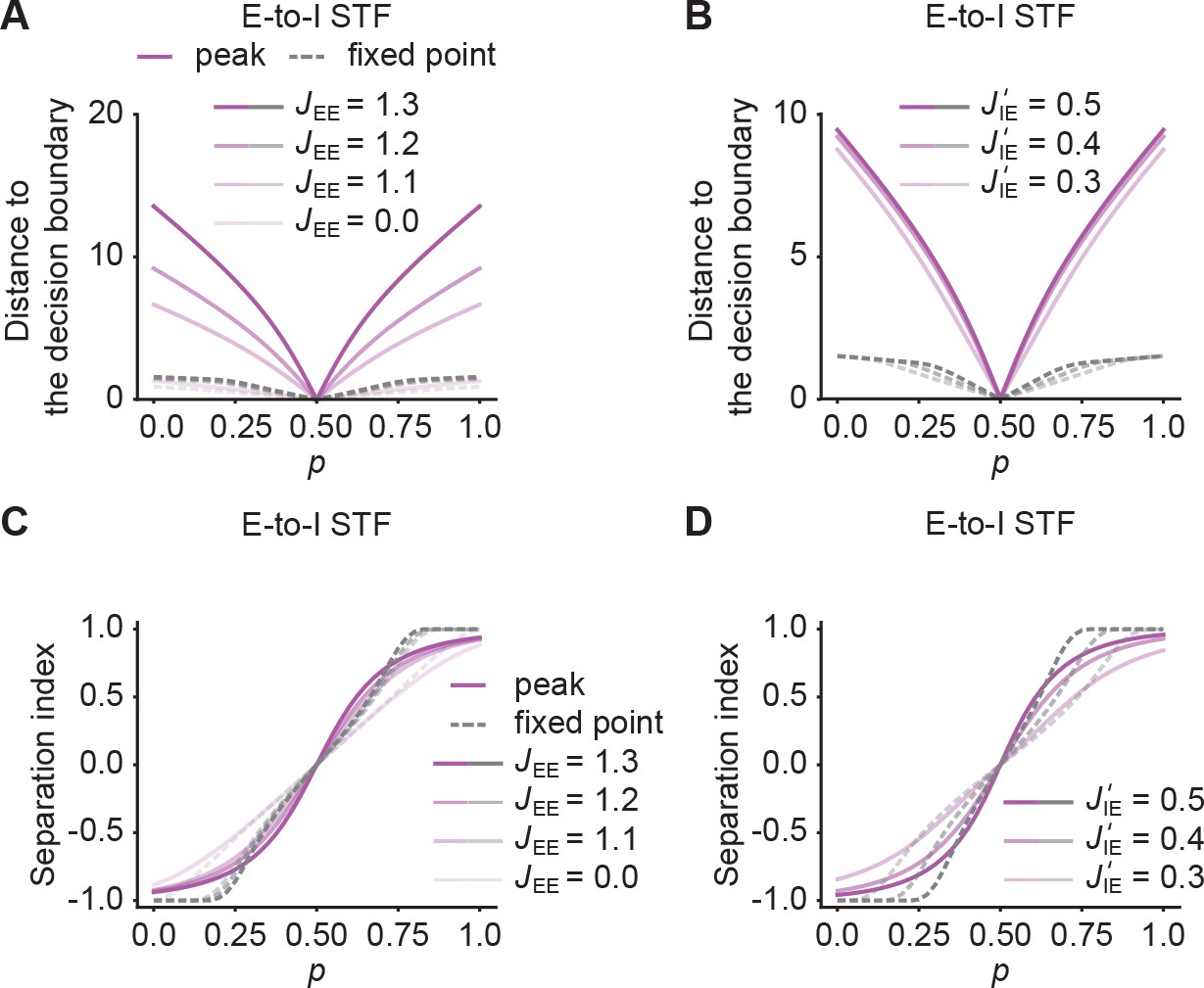
(A) Distance to the decision boundary as a function of for the peak onset response (magenta solid line) and fixed point activity (gray dashed line) for E-to-I STF. (B) Same as A but with different E-to-I connection strengths J’_IE across ensembles. (**C and D**) Same as A and B but quantified by Separation index, defined as $(r_{E 2} - r_{E 1}) / (r_{E 1} + r_{E 2})$ .

Figure 6 with 1 supplement

Download asset Open asset

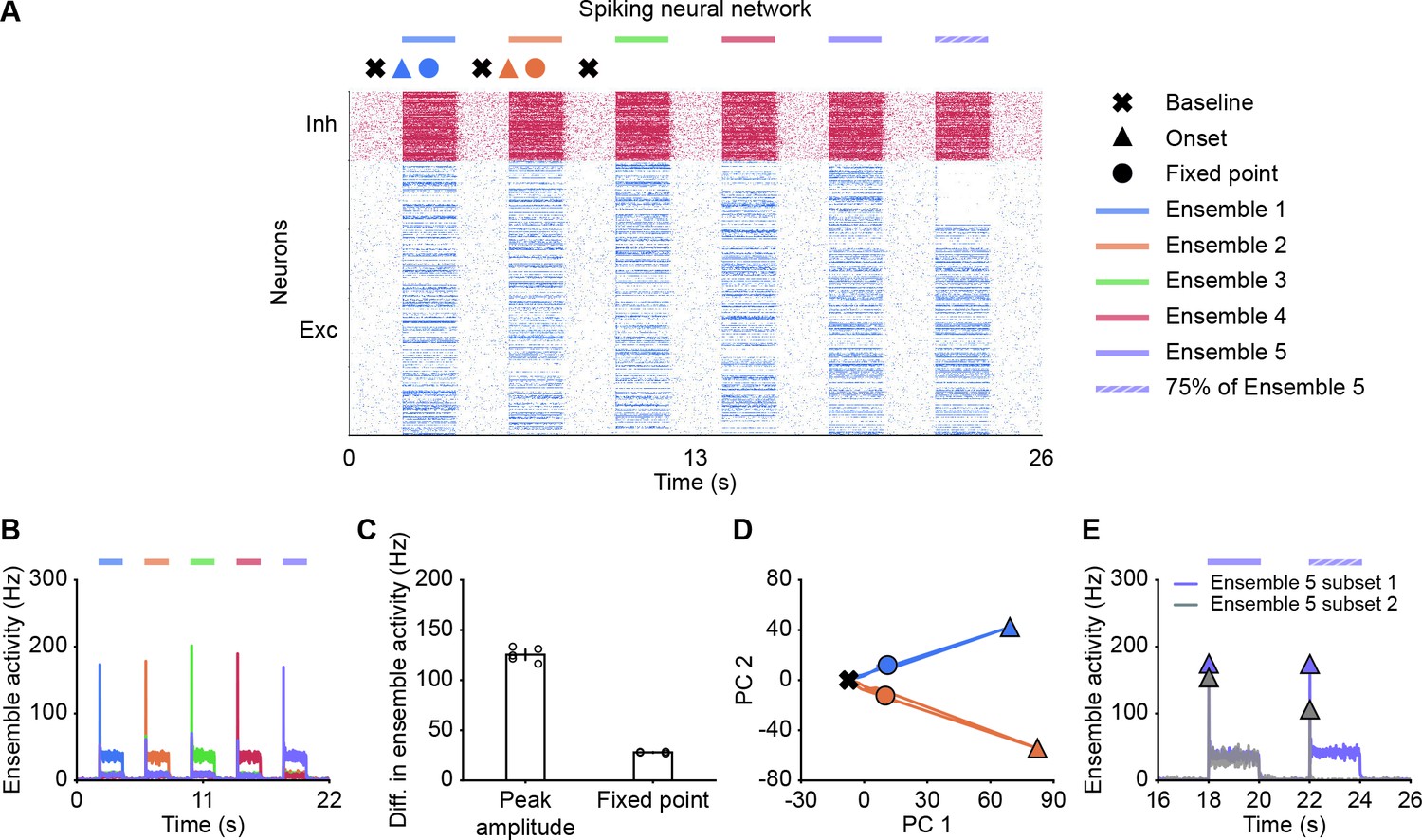
Spiking neural network simulations qualitatively reproduce NTA dynamics of rate models.

(A) Spiking activity of excitatory (blue) and inhibitory (red) neurons in a spiking neural network. From 2 to 20 s, Ensembles 1–5 individually received additional input for 2 s each (colored bars). From 22 to 24 s, 75% of Ensemble 5 neurons (Subset 1) received additional input, whereas the rest 25% of Ensemble 5 neurons (Subset 2) did not receive additional input. The symbols at the top designate the different simulation phases of baseline activity, the onset transients, and the fixed point activity. Different colors correspond to the distinct stimulation periods. (B) Ensemble activity (colors). (C) Difference in ensemble activity between the stimulated ensemble with the remaining ensembles for the transient onset peak and the fixed point. Points correspond to the different stimulation periods. (D) Spiking activity during the interval 0–10 s represented in the PCA basis spanned by the first two principal components which captured approximately 40% of the total variance. The colored lines represent the PC trajectories of the first two stimuli shown in A and B. Triangles, points and crosses correspond to the onset peak, fixed point, and baseline activity, respectively. (E) Ensemble activity of Subset 1 (purple) and Subset 2 (gray) of Ensemble 5 from 16 to 26 s. Onset peaks are marked by triangles.

Figure 6—figure supplement 1

Download asset Open asset

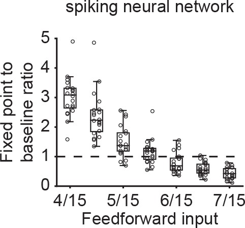
Change in steady state activity for unstimulated co-tuned neurons in spiking neural networks.

The ratio of the fixed point activity to the baseline activity for unstimulated co-tuned neurons (Ensemble 5, Subset 2) as a function of feedforward input to Subset one in spiking neural networks with E-to-E STD. The horizontal dashed line indicates a ratio of one at which the fixed point activity is identical to the baseline activity. Each point corresponds to a measurement from a randomly initialized network.

Tables

Table 1

Parameters for Figure 1C–E.

Symbol	Value	Unit	Description
$J_{E E}$	1.8	-	E-to-E connection strength
$J_{I E}$	1.0	-	E-to-I connection strength
$J_{E I}$	1.0	-	I-to-E connection strength
$J_{I I}$	0.6	-	I-to-I connection strength
$α_{E}$	2	-	Power of excitatory input-output function
$α_{I}$	2	-	Power of inhibitory input-output function
$τ_{E}$	20	ms	Time constant of excitatory firing dynamics
$τ_{I}$	10	ms	Time constant of inhibitory firing dynamics
$g_{E}^{b s}$	1.55	-	Input to the E population at baseline
$g_{E}^{s t i m}$	3.0	-	Input to the E population during stimulation
$g_{I}$	2.0	-	Input to the I population
Parameters for Figure 1F
$J_{I E}$	0.45	-	E-to-I connection strength
$J_{E I}$	1.0	-	I-to-E connection strength
$J_{I I}$	1.5	-	I-to-I connection strength

Table 2

Parameters for Figure 2.

Symbol	Value	Unit	Description
$τ_{a}$	200	ms	Time constant of SFA
$b$	1.0	-	Strength of SFA
$τ_{x}$	200	ms	Time constant of STD
$U_{d}$	1.0	-	Depression rate
$τ_{u}$	200	ms	Time constant of STF
$U_{f}$	1.0	-	Facilitation rate
$U_{m a x}$	6.0	-	Maximal facilitation value
Note that these values are also applied elsewhere unless mentioned otherwise.

Table 3

Parameters for Figure 3 bi/multi-stable example.

Symbol	Value	Unit	Description
$J_{E E}$	1.4	-	Within-ensemble E-to-E connection strength
$J_{I E}$	0.6	-	Within-ensemble E-to-I connection strength
$J_{E I}$	1.0	-	Within-ensemble I-to-E connection strength
$J_{I I}$	0.6	-	Within-ensemble I-to-I connection strength
$J_{E E}^{^{'}}$	0.14	-	Inter-ensemble E-to-E connection strength
$J_{I E}^{^{'}}$	0.6	-	Inter-ensemble E-to-I connection strength
$J_{E I}^{^{'}}$	1.0	-	Inter-ensemble I-to-E connection strength
$J_{I I}^{^{'}}$	0.6	-	Inter-ensemble I-to-I connection strength
$g_{E 1}^{b s}$	2.2	-	Input to the E1 population at baseline
$g_{E 1}^{s t i m}$	3.0	-	Input to the E1 population during stimulation
$g_{E 2}$	2.2	-	Input to the E2 population
$g_{I}$	2.0	-	Input to the I population
Parameters for Figure 3 uni-stable example
$J_{E E}$	1.3	-	Within-ensemble E-to-E connection strength
$J_{E E}^{^{'}}$	0.13	-	Inter-ensemble E-to-E connection strength

Table 4

Parameters for Figures 4 and 5.

Symbol	Value	Unit	Description
$N_{E}$	200	-	Number of excitatory neurons
$N_{I}$	50	-	Number of inhibitory neurons
$N$	2	-	Number of ensembles
$J_{E E}$	$1.2 / (N_{E} / 2 - 1)$	-	Within-ensemble E-to-E connection strength
$J_{I E}$	$1.0 / (N_{E} / 2)$	-	Within-ensemble E-to-I connection strength
$J_{E I}$	$1.0 / (N_{I} / 2)$	-	Within-ensemble I-to-E connection strength
$J_{I I}$	$1.0 / (N_{I} / 2 - 1)$	-	Within-ensemble I-to-I connection strength
$J_{E E}^{^{'}}$	$0.36 / (N_{E} / 2 - 1)$	-	Inter-ensemble E-to-E connection strength
$J_{I E}^{^{'}}$	$0.4 / (N_{E} / 2)$	-	Inter-ensemble E-to-I connection strength
$J_{E I}^{^{'}}$	$0.1 / (N_{I} / 2)$	-	Inter-ensemble I-to-E connection strength
$J_{I I}^{^{'}}$	$0.1 / (N_{I} / 2)$	-	Inter-ensemble I-to-I connection strength
$g_{I}$	2.0	-	Input to the I population
Parameters for Figure 4
$g_{E 1}^{b s}$	1.35	-	Input to the E1 population
$g_{E 1}^{s t i m}$	4.0	-	Input to the E1 population during stimulation
$g_{E 2}$	1.35	-	Input to the E2 population
Parameters for Figure 5
$g_{E 1}^{b s}$	1.35	-	Input to the E1 population at baseline
$g_{E 1}^{s t i m}$	1.35 + (4.0–1.35) (1- $p$ )	-	Input to the E1 population during stimulation
$g_{E 2}^{b s}$	1.35	-	Input to the E2 population at baseline
$g_{E 2}^{s t i m}$	1.35 + (4.0–1.35) $p$	-	Input to the E2 population during stimulation
Here, p is a parameter between 0 and 1 controlling the additional inputs to E1 and E2.

Table 5

Parameters for Figure 6.

Symbol	Value	Unit	Description
$N_{E}$	400	-	Number of excitatory neurons
$N_{I}$	100	-	Number of inhibitory neurons
$U^{rest}$	–70	mV	Resting membrane potential
$U^{exc}$	0	mV	Excitatory reversal potential
$U^{inh}$	–80	mV	Inhibitory reversal potential
$τ^{ref}$	3	ms	Duration of refractory period
$τ_{exc}^{m}$	20	ms	Membrane time constant of excitatory neurons
$τ_{inh}^{m}$	10	ms	Membrane time constant of inhibitory neurons
$τ^{ampa}$	5	ms	Time constant of AMPA receptor
$τ^{gaba}$	10	ms	Time constant of GABA receptor
$τ^{nmda}$	100	ms	Time constant of NMDA receptor
$ξ$	0.5	-	Receptor weighting factor
$J_{E E}$	0.19	-	Within-ensemble E-to-E connection strength
$J_{I E}$	0.10	-	Within-ensemble E-to-I connection strength
$J_{E I}$	0.10	-	Within-ensemble I-to-E connection strength
$J_{I I}$	0.06	-	Within-ensemble I-to-I connection strength
$J_{E E}^{^{'}}$	0.019	-	Inter-ensemble E-to-E connection strength
$J_{I E}^{^{'}}$	0.05	-	Inter-ensemble E-to-I connection strength
$J_{E I}^{^{'}}$	0.04	-	Inter-ensemble I-to-E connection strength
$J_{I I}^{^{'}}$	0.006	-	Inter-ensemble I-to-I connection strength

Appendix 5—table 1

Parameters for Figure 1—figure supplement 1.

Symbol	Value	Unit	Description
$J_{E E}$	0.5	-	E-to-E connection strength
$J_{I E}$	0.45	-	E-to-I connection strength
$J_{E I}$	1.0	-	I-to-E connection strength
$J_{I I}$	1.5	-	I-to-I connection strength
$g_{E}^{b s}$	0.5	-	Input to the E population at baseline
$g_{I}^{b s}$	1.5	-	Input to the I population at baseline

Appendix 5—table 2

Parameters for Figure 2—figure supplement 2.

Symbol	Value	Unit	Description
$g_{E}^{s t i m}$	2.0	-	Input to the E population during stimulation
Note that values of the unlisted parameters are the same as Tables 1–2.

Appendix 5—table 3

Parameters for Figure 2—figure supplement 3 SSN example.

Symbol	Value	Unit	Description
$J_{E E}$	1.8	-	E-to-E connection strength
$J_{I E}$	2.0	-	E-to-I connection strength
$J_{E I}$	1.0	-	I-to-E connection strength
$J_{I I}$	1.0	-	I-to-I connection strength

Appendix 5—table 4

Parameters for Figure 2—figure supplement 5.

Symbol	Value	Unit	Description
$g_{E}^{b s}$	1.8	-	Input to the E population at baseline
Note that values of the unlisted parameters are the same as Tables 1–2.

Appendix 5—table 5

Parameters for Figure 2—figure supplement 10.

Symbol	Value	Unit	Description
$N_{E}$	400	-	Number of excitatory neurons
$N_{I}$	100	-	Number of inhibitory neurons
$J_{E E}$	0.05	-	E-to-E connection strength
$J_{I E}$	0.02	-	E-to-I connection strength
$J_{E I}$	0.05	-	I-to-E connection strength
$J_{I I}$	0.03	-	I-to-I connection strength

Appendix 5—table 6

Parameters for Figure 2—figure supplement 11.

Symbol	Value	Unit	Description
$J_{E E}$	0.9	-	E-to-E connection strength
$J_{I E}$	1.2	-	E-to-I connection strength
$J_{E I}$	0.5	-	I-to-E connection strength
$J_{I I}$	0.5	-	I-to-I connection strength
$τ_{E}$	20	ms	Time constant of excitatory firing dynamics
$τ_{I}$	60	ms	Time constant of inhibitory firing dynamics
$g_{E}^{b s}$	1.0	-	Input to the E population at baseline
$g_{E}^{s t i m}$	2.0	-	Input to the E population during stimulation
$g_{I}$	2.0	-	Input to the I population
Note that values of the unlisted parameters are the same as Tables 1–2.

Appendix 5—table 7

Parameters for Figure 2—figure supplement 12.

Symbol	Value	Unit	Description
$J_{E E}$	1.0	-	E-to-E connection strength
$J_{I E}$	1.2	-	E-to-I connection strength
$J_{E I}$	0.5	-	I-to-E connection strength
$J_{I I}$	1.0	-	I-to-I connection strength
$g_{E}^{b s}$	0.5	-	Input to the E population at baseline
$g_{I}^{b s}$	1.0	-	Input to the I population at baseline

Appendix 5—table 8

Parameters for Figure 3—figure supplement 1 global inhibition example.

Symbol	Value	Unit	Description
$J_{E E}$	1.6	-	Within-ensemble E-to-E connection strength
$J_{I E}$	1.0	-	Within-ensemble E-to-I connection strength
$J_{E I}$	1.0	-	Within-ensemble I-to-E connection strength
$J_{I I}$	1.2	-	Within-ensemble I-to-I connection strength
$J_{E E}^{^{'}}$	0.16	-	Inter-ensemble E-to-E connection strength
$J_{I E}^{^{'}}$	1.0	-	Inter-ensemble E-to-I connection strength
$J_{E I}^{^{'}}$	1.0	-	Inter-ensemble I-to-E connection strength
$J_{I I}^{^{'}}$	1.2	-	Inter-ensemble I-to-I connection strength
$g_{E 1}^{b s}$	1.5	-	Input to the E1 population at baseline
$g_{E 2}$	1.5	-	Input to the E2 population
$g_{I 1}$	2.5	-	Input to the I1 population
$g_{I 2}$	2.5	-	Input to the I2 population
Parameters for Figure 3—figure supplement 1 co-tuned example
$J_{I E}$	1.0 * (4/3)	-	Within-ensemble E-to-I connection strength
$J_{E I}$	1.0 * (4/3)	-	Within-ensemble I-to-E connection strength
$J_{I I}$	1.2 * (4/3)	-	Within-ensemble I-to-I connection strength
$J_{I E}^{^{'}}$	1.0 * (2/3)	-	Inter-ensemble E-to-I connection strength
$J_{E I}^{^{'}}$	1.0 * (2/3)	-	Inter-ensemble I-to-E connection strength
$J_{I I}^{^{'}}$	1.2 * (2/3)	-	Inter-ensemble I-to-I connection strength

Appendix 5—table 9

Parameters for Figure 4—figure supplement 1.

Symbol	Value	Unit	Description
$J_{E E}$	$1.5 / (N_{E} / 2 - 1)$	-	Within-ensemble E-to-E connection strength
$J_{I E}$	$1.0 / (N_{E} / 2)$	-	Within-ensemble E-to-I connection strength
$J_{E I}$	$1.0 / (N_{I} / 2)$	-	Within-ensemble I-to-E connection strength
$J_{I I}$	$1.0 / (N_{I} / 2 - 1)$	-	Within-ensemble I-to-I connection strength
$J_{E E}^{^{'}}$	$0.1 / (N_{E} / 2 - 1)$	-	Inter-ensemble E-to-E connection strength
$J_{I E}^{^{'}}$	$0.3 / (N_{E} / 2)$	-	Inter-ensemble E-to-I connection strength
$J_{E I}^{^{'}}$	$0.3 / (N_{I} / 2)$	-	Inter-ensemble I-to-E connection strength
$J_{I I}^{^{'}}$	$0.1 / (N_{I} / 2)$	-	Inter-ensemble I-to-I connection strength
$g_{E 1}^{b s}$	1.5	-	Input to the E1 population at baseline
$g_{E 2}$	1.5	-	Input to the E2 population
$g_{I}$	2.0	-	Input to the I population

Appendix 5—table 10

Parameters for Figure 6—figure supplement 1.

Symbol	Value	Unit	Description
$J_{E E}$	0.20	-	Within-ensemble E-to-E connection strength
$J_{I E}$	0.09	-	Within-ensemble E-to-I connection strength
$J_{E I}$	0.10	-	Within-ensemble I-to-E connection strength
$J_{I I}$	0.10	-	Within-ensemble I-to-I connection strength
$J_{E E}^{^{'}}$	0.02	-	Inter-ensemble E-to-E connection strength
$J_{I E}^{^{'}}$	0.054	-	Inter-ensemble E-to-I connection strength
$J_{E I}^{^{'}}$	0.07	-	Inter-ensemble I-to-E connection strength
$J_{I I}^{^{'}}$	0.01	-	Inter-ensemble I-to-I connection strength
Note that values of the unlisted parameters are the same as Table 5.

Additional files

Transparent reporting form: https://cdn.elifesciences.org/articles/71263/elife-71263-transrepform1-v2.pdf
Download elife-71263-transrepform1-v2.pdf

Download links

A two-part list of links to download the article, or parts of the article, in various formats.

Downloads (link to download the article as PDF)

Open citations (links to open the citations from this article in various online reference manager services)

Mendeley

Cite this article (links to download the citations from this article in formats compatible with various reference manager tools)

Yue Kris Wu
Friedemann Zenke

(2021)

Nonlinear transient amplification in recurrent neural networks with short-term plasticity

eLife 10:e71263.

https://doi.org/10.7554/eLife.71263

Share this article

Cite this article

Neuronal ensembles nonlinearly amplify inputs above a critical threshold.

Unstable ensemble dynamics can be triggered by additional stimulation in supralinear networks with negative determinant even in the presence of substantial feedforward inhibition.

Short-term plasticity, but not spike-frequency adaptation, re-stabilizes ensemble dynamics.

Ensemble dynamics in supralinear networks with strong SFA.

Dependence of peak amplitude and fixed point activity on input gE and E-to-E connection strength JEE.

Comparisons of amplification ability between NTA and linear networks, and between NTA and SSNs.

Dependence of peak amplitude and fixed point activity on STP parameters.

Networks initially in the ISN regime can exhibit strong NTA.

ISN index and paradoxical effect test for networks with E-to-I STF.

Inhibition stabilization does not imply paradoxical response in networks with E-to-E STD.

Transition from non-ISN to ISN indicating by frozen inhibition test.

Similar qualitative behavior in rate-based models with maximal firing rate capped at 300 Hz.

Similar qualitative behavior in spiking neural networks.

Unstable dynamics can emerge in supralinear networks with positive determinant and slow inhibition.

Networks with substantial feedforward inhibition can exhibit strong NTA.

Co-tuned inhibition broadens the parameter regime of NTA in the absence of persistent activity.

Ensembles with co-tuned inhibition exhibit weaker — but still strong — NTA in comparison to ensembles with global inhibition.

NTA yields stronger pattern completion than fixed points while retaining stimulus selectivity.

Change in steady state activity for unstimulated co-tuned neurons in the rate-based model.

Quantification of pattern completion and stimulus selectivity in networks with E-to-I STF.

NTA provides stronger amplification and pattern separation in morphing experiments than fixed point activity.

Quantification of pattern separation in morphing experiments using a normalized measure.

Quantification of pattern separation in morphing experiments for networks with E-to-I STF.

Spiking neural network simulations qualitatively reproduce NTA dynamics of rate models.

Change in steady state activity for unstimulated co-tuned neurons in spiking neural networks.

Parameters for Figure 1C–E.

Parameters for Figure 2.

Parameters for Figure 3 bi/multi-stable example.

Parameters for Figures 4 and 5.

Parameters for Figure 6.

Parameters for Figure 1—figure supplement 1.

Parameters for Figure 2—figure supplement 2.

Parameters for Figure 2—figure supplement 3 SSN example.

Parameters for Figure 2—figure supplement 5.

Parameters for Figure 2—figure supplement 10.

Parameters for Figure 2—figure supplement 11.

Parameters for Figure 2—figure supplement 12.

Parameters for Figure 3—figure supplement 1 global inhibition example.

Parameters for Figure 4—figure supplement 1.

Parameters for Figure 6—figure supplement 1.

Transparent reporting form

Downloads (link to download the article as PDF)

Open citations (links to open the citations from this article in various online reference manager services)

Cite this article (links to download the citations from this article in formats compatible with various reference manager tools)

Dependence of peak amplitude and fixed point activity on input g_E and E-to-E connection strength J_EE.