Extent, impact, and mitigation of batch effects in tumor biomarker studies using tissue microarrays
- Department of Epidemiology, Harvard T.H. Chan School of Public Health, United States
- Department of Medicine, Memorial Sloan Kettering Cancer Center, United States
- Department of Biostatistics, Harvard T.H. Chan School of Public Health, United States
- Department of Data Science, Dana-Farber Cancer Institute, United States
- Channing Division of Network Medicine, Department of Medicine, Brigham and Women’s Hospital and Harvard Medical School, United States
- Department of Cancer Epidemiology, Moffitt Cancer Center, United States
- Department of Pathology, St. James’s Hospital, Ireland
- Trinity College, Ireland
- Pathology Unit, Addarii Institute, S. Orsola-Malpighi Hospital, Italy
- Department of Pathology, Weill Cornell Medical College, United States
- Department of Pathology, Johns Hopkins Medical Institutions, United States
Figures
Figure 1
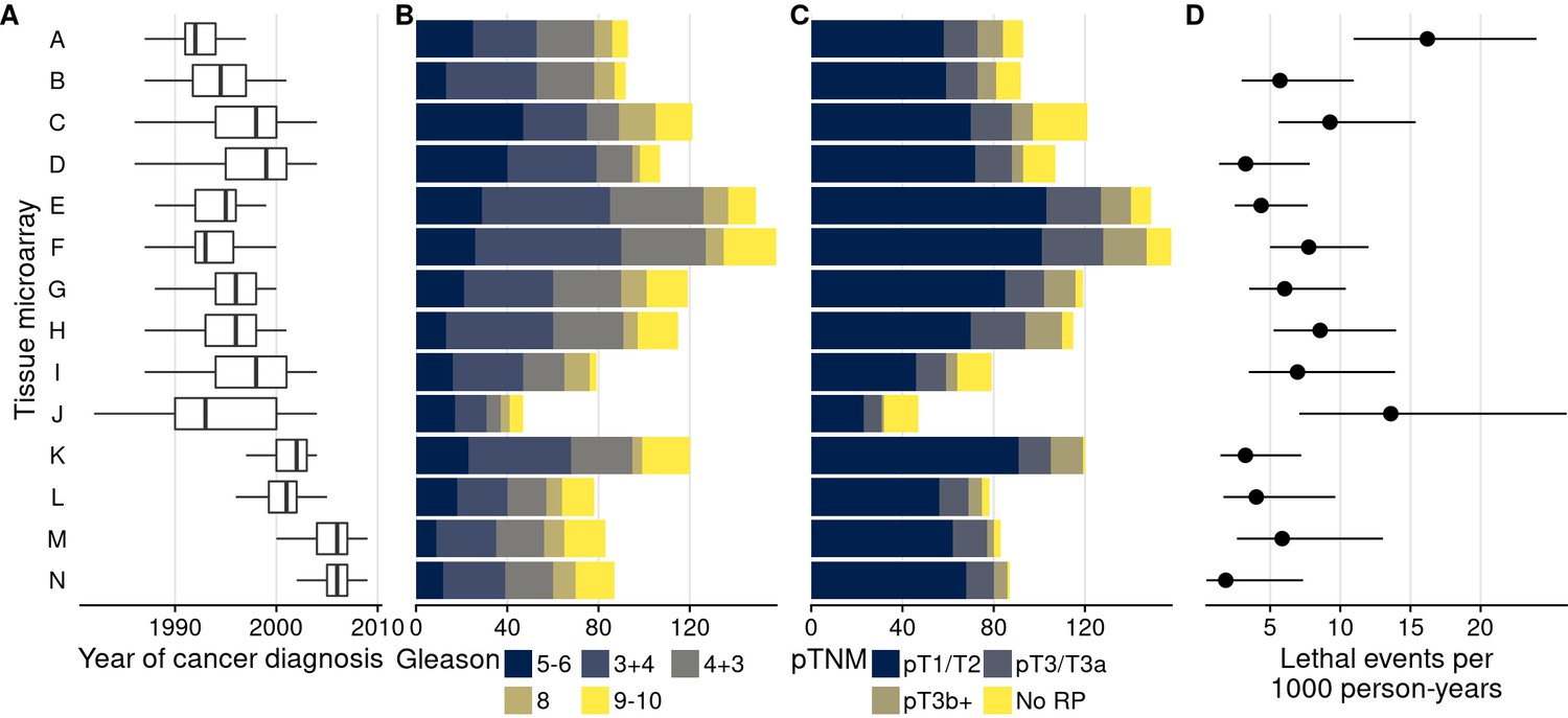
Characteristics of men with prostate cancer with tissue included on the 14 tumor tissue microarrays.
(A) Calendar years of cancer diagnosis, with thick lines indicating median, boxes interquartile ranges, and whiskers 1.5 times the interquartile range. (B) Counts of tumors by Gleason score. (C) Counts of tumors by pathological TNM stage (RP: radical prostatectomy). (D) Rates of lethal disease (metastases or prostate cancer-specific death over long-term follow-up), with bars indicating 95% confidence intervals. As throughout, multiple cores are summarized per tumor.
Figure 2 with 1 supplement
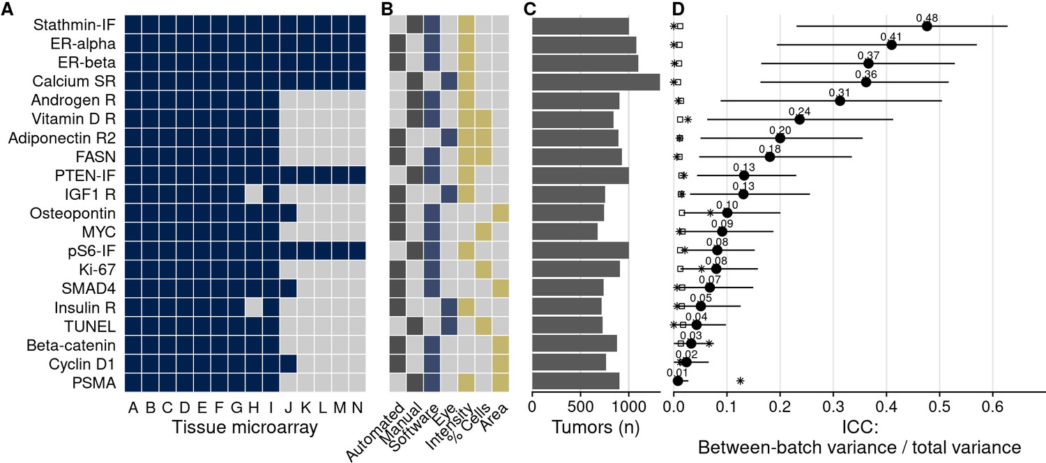
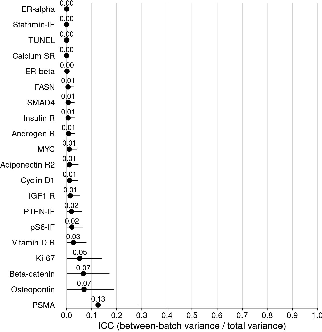
Biomarkers stained, staining and scoring methods, and intraclass correlation coefficients (ICCs).
(A) Tissue microarrays (TMAs) assessed for each marker (dark blue, yes). (B) Approach to staining biomarkers: automated staining system versus manual staining (gray, yes); quantification of biomarkers: software-based scoring versus eye scoring (blue, yes); biomarker quality assessed: staining intensity, proportion of cells positive for the biomarker, area of tissue positive for the biomarker (yellow, yes). (C) Counts of tumors assessed for each biomarker. (D) Between-TMA ICCs (i.e., proportion of variance explained by between-TMA differences) for each biomarker, with 95% confidence intervals. Empty symbols indicate the 97.5th percentile of the null distribution of the ICC obtained by permuting tumor assignments to TMAs; asterisks indicate between-Gleason grade group ICCs. Biomarkers are arranged by descending between-TMA ICC.
Figure 2—figure supplement 1
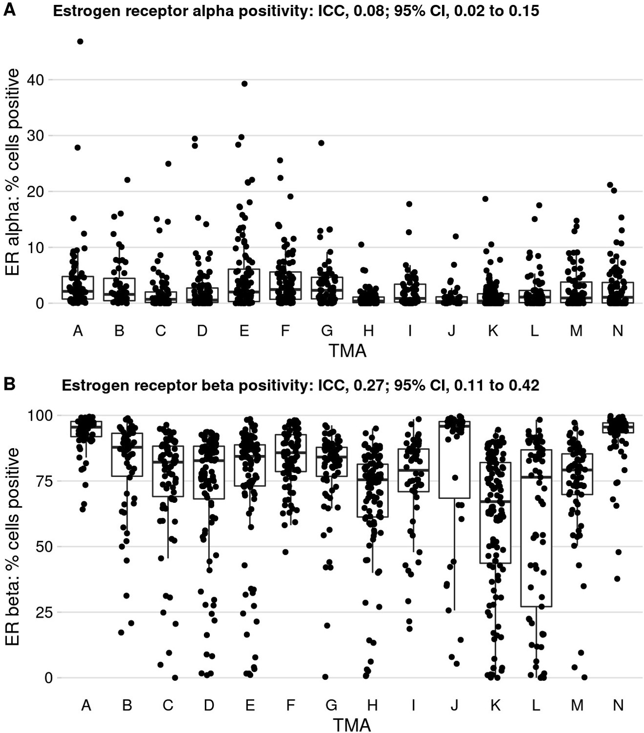
Tissue microarrays (TMAs) and differences in % positivity, at the example of estrogen receptor alpha and beta, and variance in biomarker levels explained by between-TMA differences (ICC).
ICC, intraclass correlation coefficient.
Figure 3 with 1 supplement
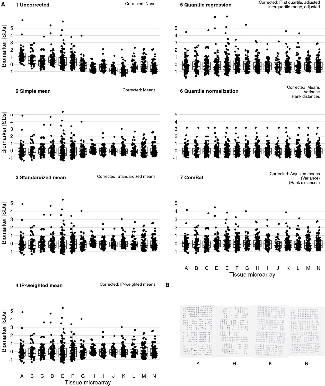
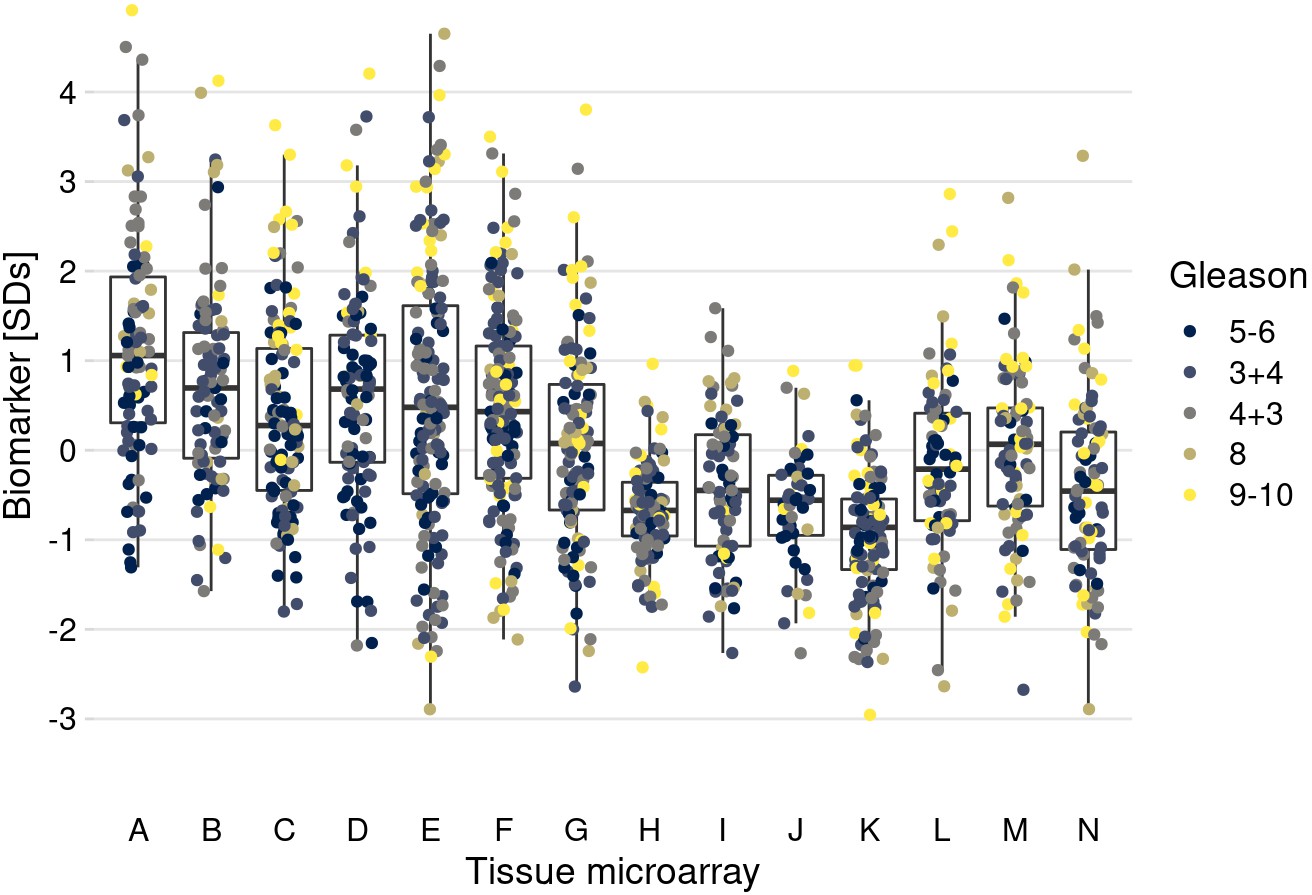
Effect of batch effect mitigation on a biomarker with strong between-tissue microarray (TMA) variation.
(A) The protein biomarker estrogen receptor-alpha was quantified as staining intensity in nuclei of epithelial cells, averaged over all cores of each tumor. Each panel shows processed data for a specific approach to correcting batch effects. Notes in the upper right corner indicate which properties of batch effects were potentially addressed. Each data point represents one tumor. y-axes are standard deviations of the combined data for the specific method. Thick lines indicate medians, boxes interquartile ranges, and whisker length is 1.5 times the interquartile range. (B) Example photographs of TMAs; brown color indicates positive staining.
Figure 3—figure supplement 1
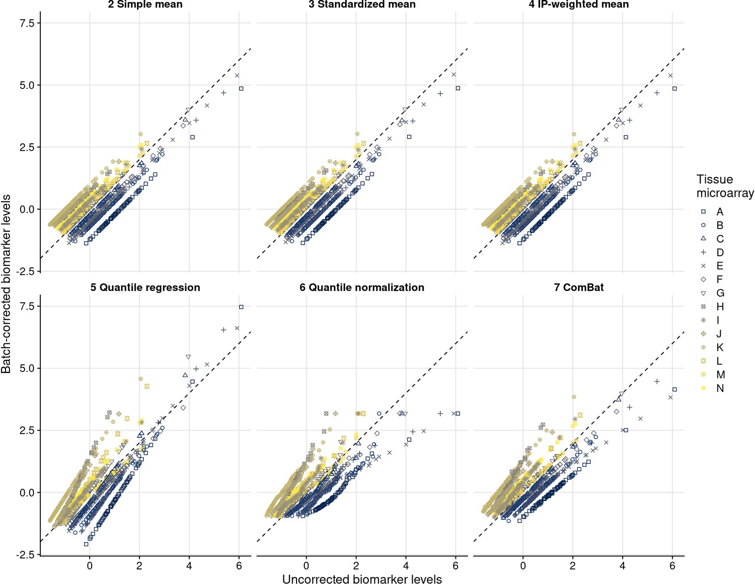
Uncorrected compared with batch effect-corrected biomarker levels for estrogen receptor alpha.
Symbols and color indicate the tissue microarray.
Figure 4 with 7 supplements
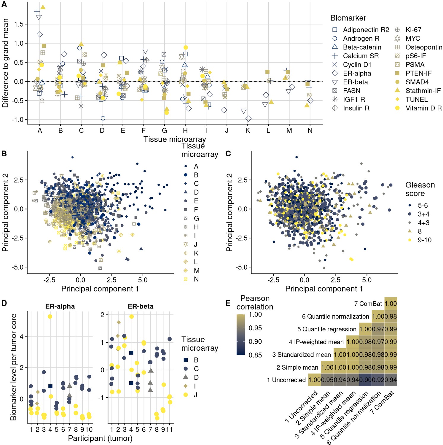
Patterns, source, and remediation of batch effects.
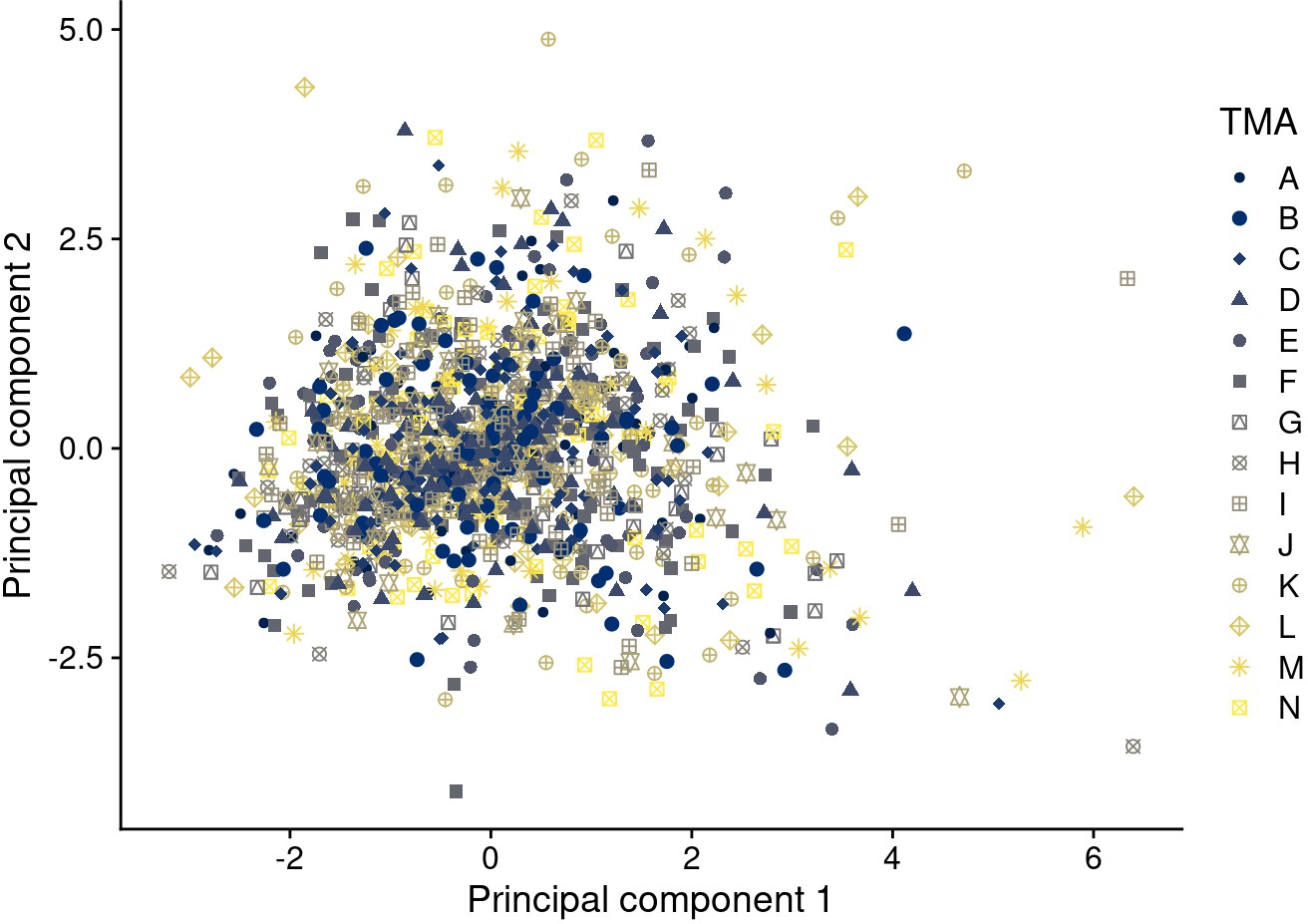
(A), Biomarker mean levels by tissue microarray (TMA), in biomarker-specific standard deviations (y-axis). Each point is one TMA. (B) First two principal components of biomarkers levels on all 14 TMAs, with color/shape denoting TMA. Each point is one tumor. (C) The same first two principal components, with color/shape denoting Gleason score. (D) Per-core biomarker levels for tumors with multiple cores included on two separate TMAs, for estrogen receptor (ER) alpha and beta, both in standard deviations. Each point is one tumor core. (E) Pearson correlation coefficients r between uncorrected and corrected biomarker levels. Entries are averages across all markers.
Figure 4—figure supplement 1
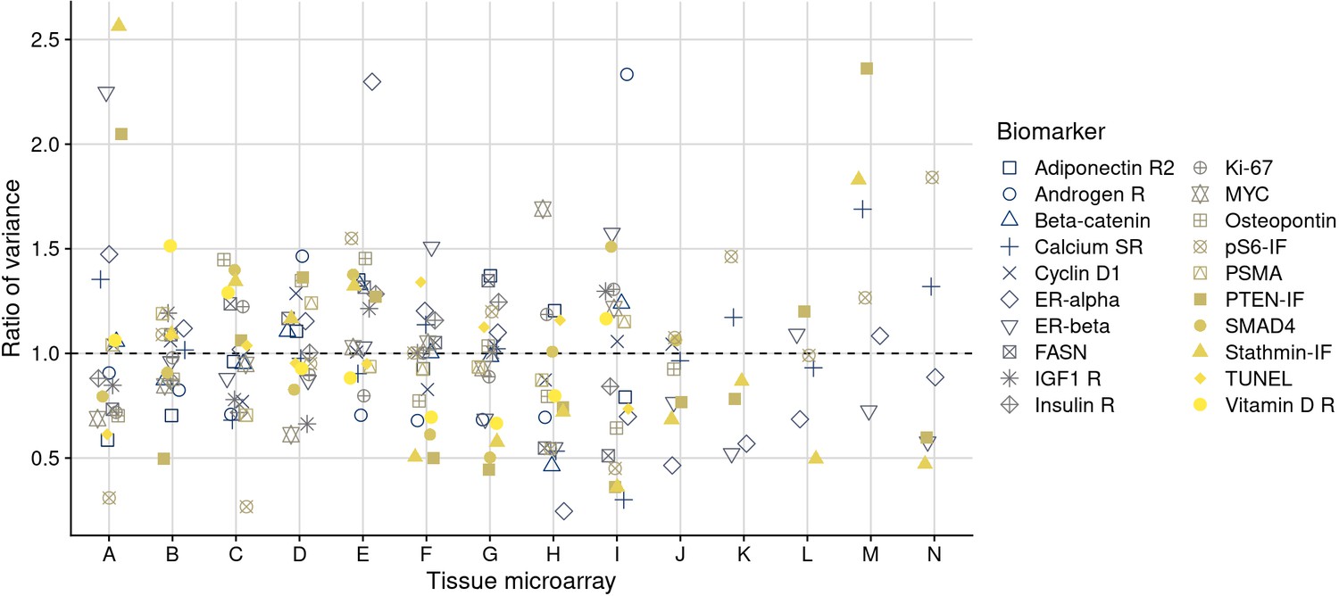
Ratios of variance per tissue microarray to the mean variance for each marker.
Figure 4—figure supplement 2
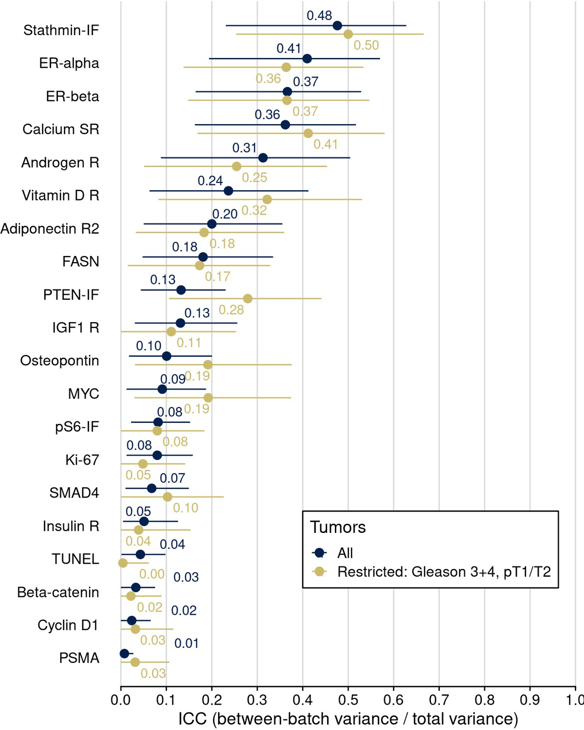
Intraclass correlation coefficients (ICCs), quantifying the proportion of variance in biomarker levels attributable to between-tissue microarray (TMA) differences, across all tumors and after restriction to those 378 tumors across TMAs that have the same clinical/pathological characteristics in terms of Gleason score 3+4 and prostatectomy stage pT1/T2.
Figure 4—figure supplement 3
Intraclass correlation coefficients (ICCs), quantifying the proportion of variance in biomarker levels attributable to between-Gleason grade differences, sorted by increasing ICC.
Figure 4—figure supplement 4
Principal components 1 and 2 after batch effect correction using quantile normalization (approach 6) for biomarkers available on all tissue microarrays (TMAs).
Symbol color and shape indicate the TMA.
Figure 4—figure supplement 5
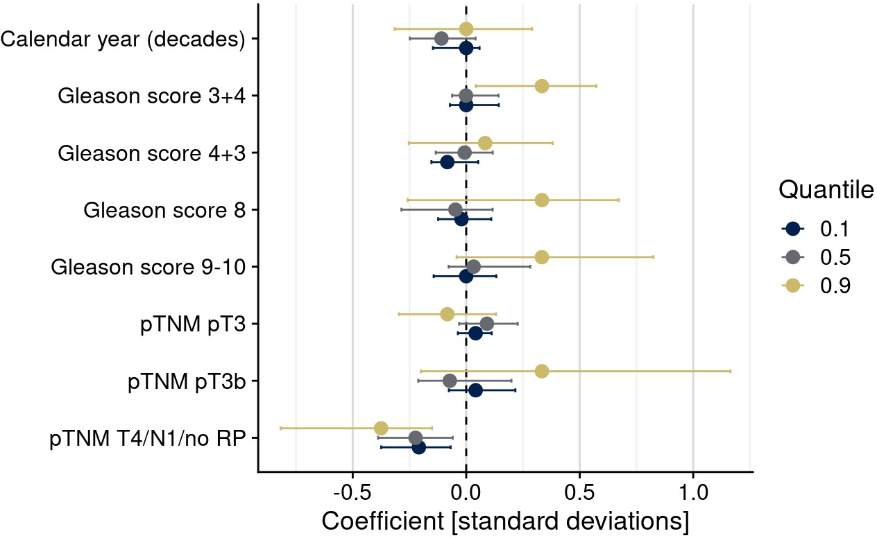
Quantile-specific associations of confounders (clinical/pathological differences) with (uncorrected) biomarker levels of estrogen receptor alpha.
Shown are regression coefficients for the 10th, 50th, and 90th percentiles as the outcomes of quantile regression models.
Figure 4—figure supplement 6
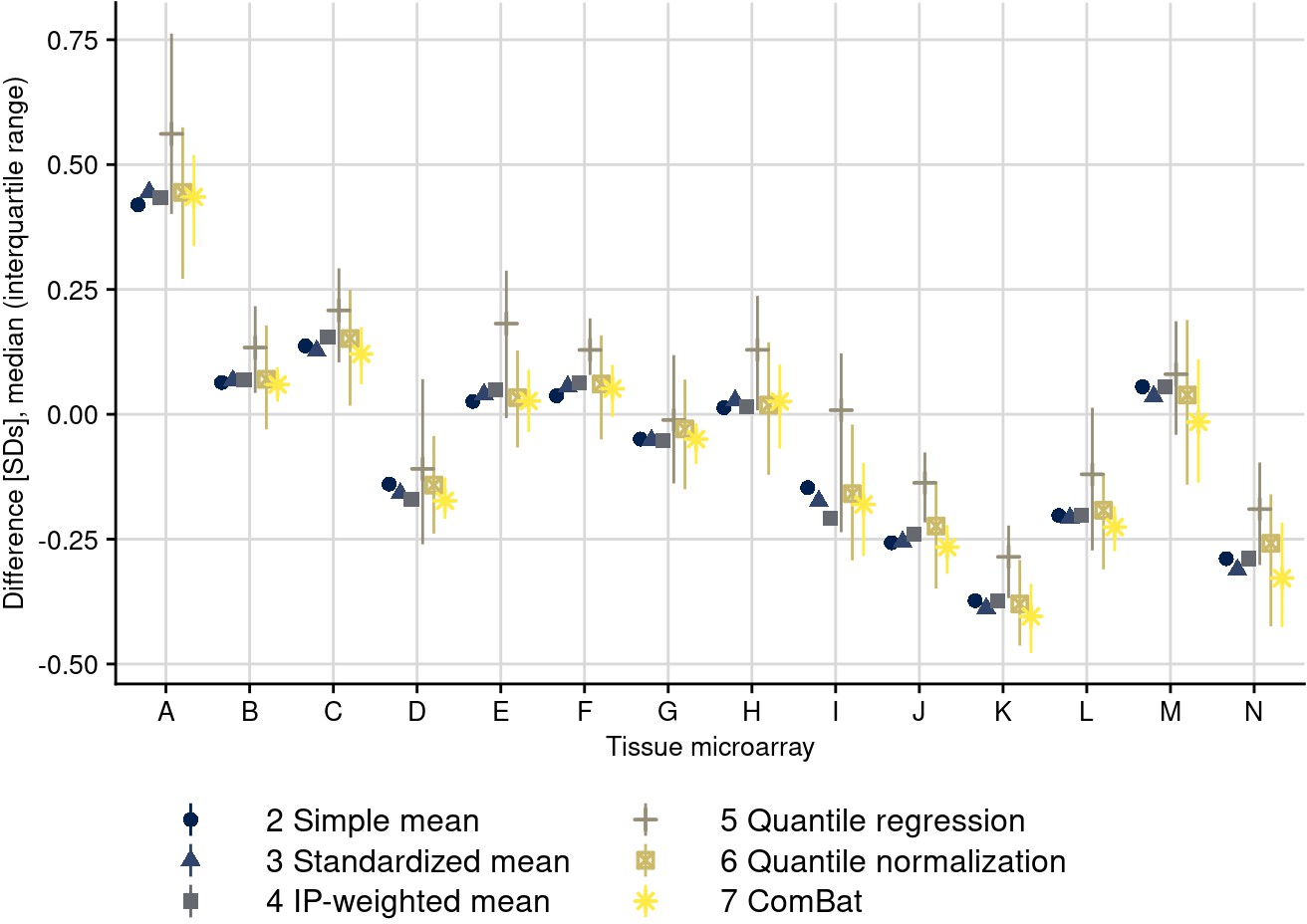
Batch corrections per tissue microarray and method.
The plot shows the difference between uncorrected and corrected values per batch, averaged across all biomarkers. IGF1-R was excluded because of missing values for some correction approaches. For batch correction approaches that only address the mean (i.e., that subtract the same correction value from all biomarker values within each batch), only that difference is visible; for correction methods that address individual values within batches differently, batch-specific medians and interquartile ranges of differences between uncorrected and corrected values are visible.
Figure 4—figure supplement 7
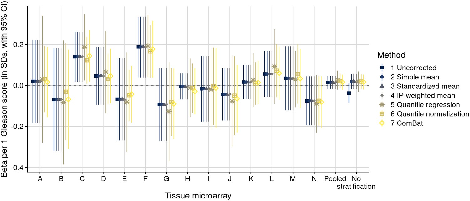
Biomarker differences in ER-alpha intensity, after batch effect correction methods, for a one-unit increment in Gleason score, stratified by tissue microarray (TMA).
“Pooled” indicates estimates pooled over batches (TMAs) using inverse-variance weighting. “No stratification” indicates estimates without stratification.
Figure 5 with 3 supplements
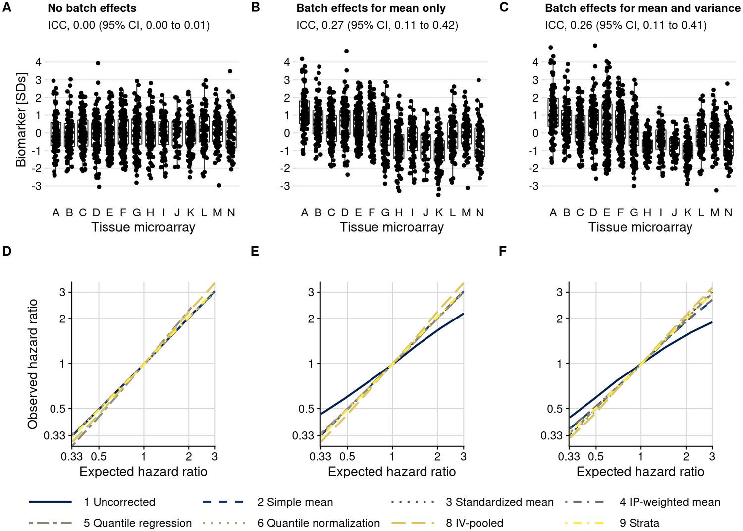
Plasmode simulation results.
(A–C) Biomarker levels by tissue microarray in three simulation scenarios. (D–F) True versus observed hazard ratios for the biomarker–outcome association after alternative approaches to batch effect correction, with correction methods being numbered as in the Materials and methods section. The solid blue line indicates no correction for batch effects. (A, D) no batch effects; (B, E) means-only batch effects; (C, F) means and variance batch effects.
Figure 5—figure supplement 1
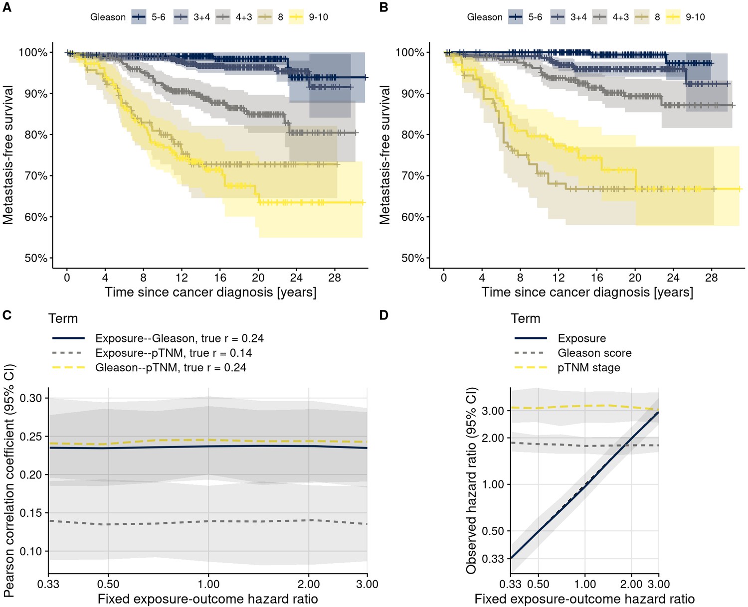
Data structures in the actual data and in 200 plasmode simulation data sets.
(A) Gleason scores and lethal prostate cancer (metastasis-free survival) in the actual data. (B) Gleason scores and lethal prostate cancer in an example simulated data set. Shaded areas indicate 95% confidence intervals. (C) Pearson correlation coefficients between biomarker levels and confounders, and between confounders, across all simulated datasets. Correlation coefficients observed in the actual data are noted in the legend. (D) Hazard ratios for the biomarker and the confounders in relation to lethal prostate cancer, pooling all simulated data sets. Confounder–outcome associations were simulated to correspond to their observed values in the actual data; exposure–outcome associations were simulated to a range of hazard ratios (x-axis). Lines indicate medians across simulations with the same exposure–outcome hazard ratio, shaded areas range from the 2.5th to 97.5th percentile.
Figure 5—figure supplement 2
The data correlation structure “confounding and imbalance."
Tumors with more extreme Gleason scores were set to be more extremely influenced by batch effects in terms of mean and variances.
Figure 5—figure supplement 3
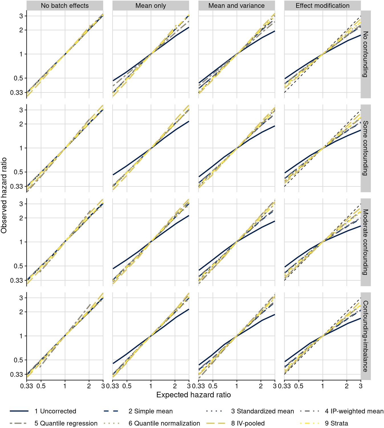
Plasmode simulation results for all scenarios.
Observed hazard ratios after different approaches to batch effect correction (y-axis) are compared to true (fixed) hazard ratios for the biomarker–outcome association (x-axis; solid blue line: no correction for batch effects). Columns are different batch effects that were added; rows are different data correlation structures.
Figure 6

Consequences of batch effect mitigation on scientific inference.
(A) Gleason score and biomarker levels (in standard deviations, per Gleason grade group). (B) Biomarker levels and progression to lethal disease, with hazard ratios per one standard deviation increase in biomarker levels from univariable Cox regression models. In both panels, blue dots indicate estimates using uncorrected biomarker levels, yellow dots indicate batch effect-corrected levels, applying quantile normalization (approach 6). Lines are 95% confidence intervals. Biomarkers are ordered by decreasing between-tissue microarray intraclass correlation coefficient (ICC).
Figure 7
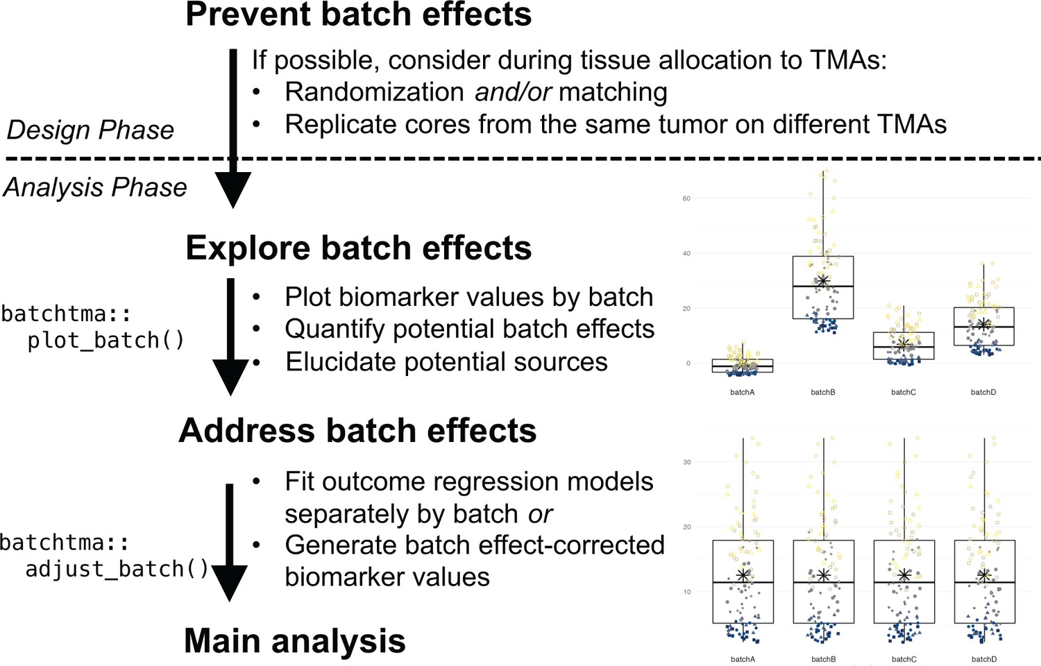
Recommended workflow for anticipating and handling batch effects between tissue microarrays (TMAs).
Following prevention approaches at the design phase of a project, all TMA-based studies should explore the potential for batch effects once a biomarker has been measured. Addressing batch effects should only be skipped there is no indication for their presence. Batch effect-corrected biomarker levels can easily be generated by the batchtma R package.
Additional files
-
Supplementary file 1
Tables, Figures, and Source Code.
(a) Interaction terms to test for multiplicative effect modification, that is whether batch effects more strongly affect tumors with more extreme clinical/pathological characteristics. The table shows point estimates (differences in biomarker levels), 95% confidence interval bounds, p-values, and false-discovery rates (FDR, in ascending order) for interaction terms between the within-batch normalized biomarker level and the potential effect modifier in linear models that have absolute biomarker levels in standard deviation units per biomarker as the outcome and also include main effects for the biomarker and the effect modifier (terms not shown). (b) ICC for between-batch variance for uncorrected biomarker levels (“1 Raw”) and biomarker levels after applying different correction methods. (c) Results from plasmode simulation according to type of induced batch effect, using the data correlation structure “moderate confounding.” For three fixed (“true”) hazard ratios for the biomarker–outcome association (1/3, 1, and 3), the observed hazard ratios after batch correction (with 95% confidence intervals) are shown. (d) Results from plasmode simulation according to data correlation structure, using the batch effect “mean and variance.” For three fixed (“true”) hazard ratios for the biomarker–outcome association (1/3, 1, and 3), the observed hazard ratios after batch correction (with 95% confidence intervals) are shown. (e) Gleason grade—biomarker associations according to batch effect correction method. Point estimates from unadjusted linear regression models for biomarker values with Gleason score categories per 1 “grade group” increase as the predictor are shown (with 95% confidence intervals). For loge-transformed markers like Ki-67, estimates are differences on the loge scale. (f) Biomarker levels and lethal disease according to batch effect correction method. Hazard ratios (with 95% confidence intervals) per one standard deviation increase in the biomarker (linear) from unadjusted Cox regression models are shown. (g) Biomarker levels and lethal disease according to batch effect correction method. Unlike in the preceding table, the hazard ratios (with 95% confidence intervals) are contrasts comparing extreme quartiles (fourth compared to first quartile) from unadjusted Cox regression models.
- https://cdn.elifesciences.org/articles/71265/elife-71265-supp1-v3.docx
-
Transparent reporting form
- https://cdn.elifesciences.org/articles/71265/elife-71265-transrepform1-v3.pdf
-
Source code 1
Analytical code and output in R Markdown format that produced all figures, figure supplements, tables, and data mentioned in the text.
- https://cdn.elifesciences.org/articles/71265/elife-71265-code1-v3.zip
Download links
A two-part list of links to download the article, or parts of the article, in various formats.
Downloads (link to download the article as PDF)
Open citations (links to open the citations from this article in various online reference manager services)
Cite this article (links to download the citations from this article in formats compatible with various reference manager tools)
Extent, impact, and mitigation of batch effects in tumor biomarker studies using tissue microarrays
eLife 10:e71265.
https://doi.org/10.7554/eLife.71265


