Figures and data in How to assemble a scale-invariant gradient | eLife

Version of Record

Accepted for publication after peer review and revision.

Download
Cite
Share
CommentOpen annotations (there are currently 0 annotations on this page).

Version of Record published: April 6, 2022 (This version)
Accepted Manuscript published: March 21, 2022 (Go to version)
Accepted: March 20, 2022
Received: June 17, 2021
Preprint posted: May 20, 2021 (Go to version)

Figures
Additional files

10 figures and 1 additional file

Figures

Figure 1

Download asset Open asset

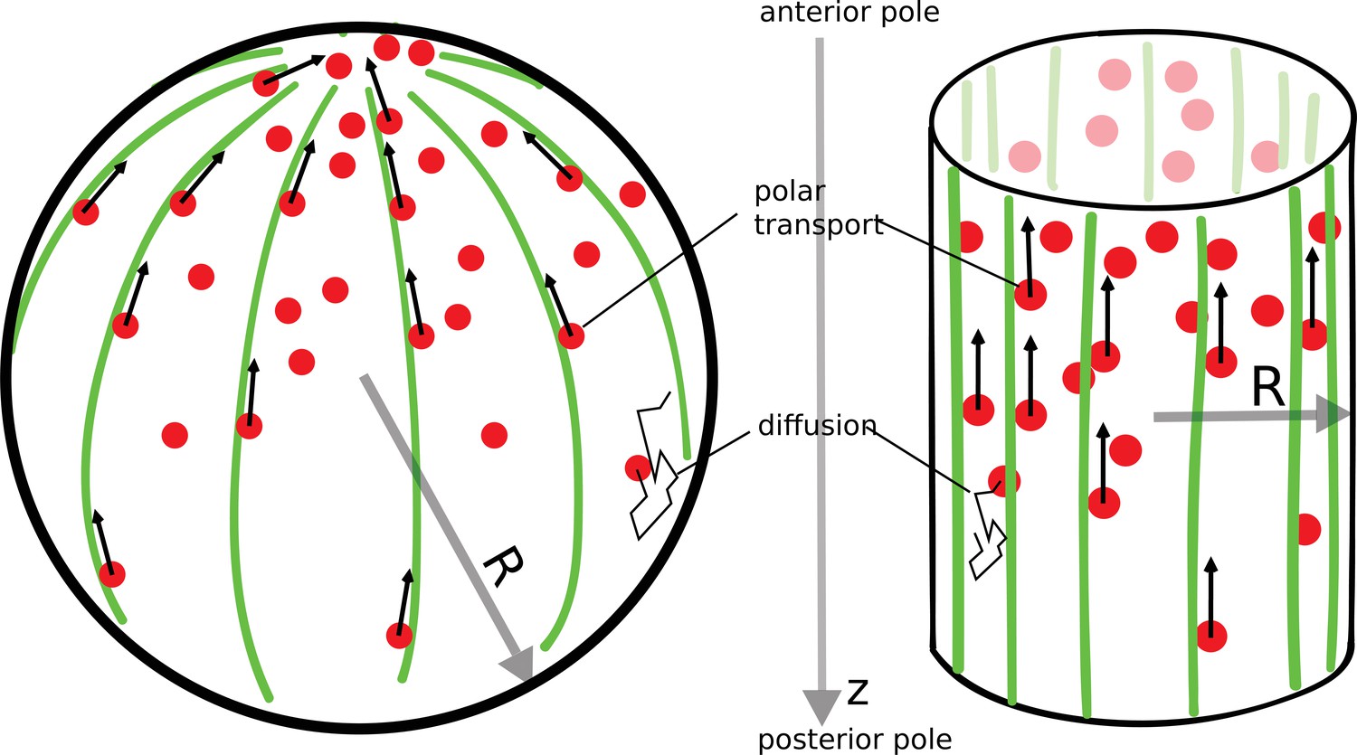
The polar transport model of gradient formation.

Transport of proteins (red) in the cell is a combination of diffusion and polar transport. Diffusion occurs throughout the cytoplasm. When diffusing proteins encounter motor proteins (black arrows) moving along polar filaments (green) that contour the cell surface, they can be taken up by the motors and delivered to the cell’s anterior pole. The anterior pole acts as a source, while the filaments along the surface of the cell serve as a sink of diffusing proteins. The result of this combined polar transport and diffusion is a protein gradient that extends along the polar ( $z$ ) axis of the cell, with proteins accumulating toward the anterior pole.

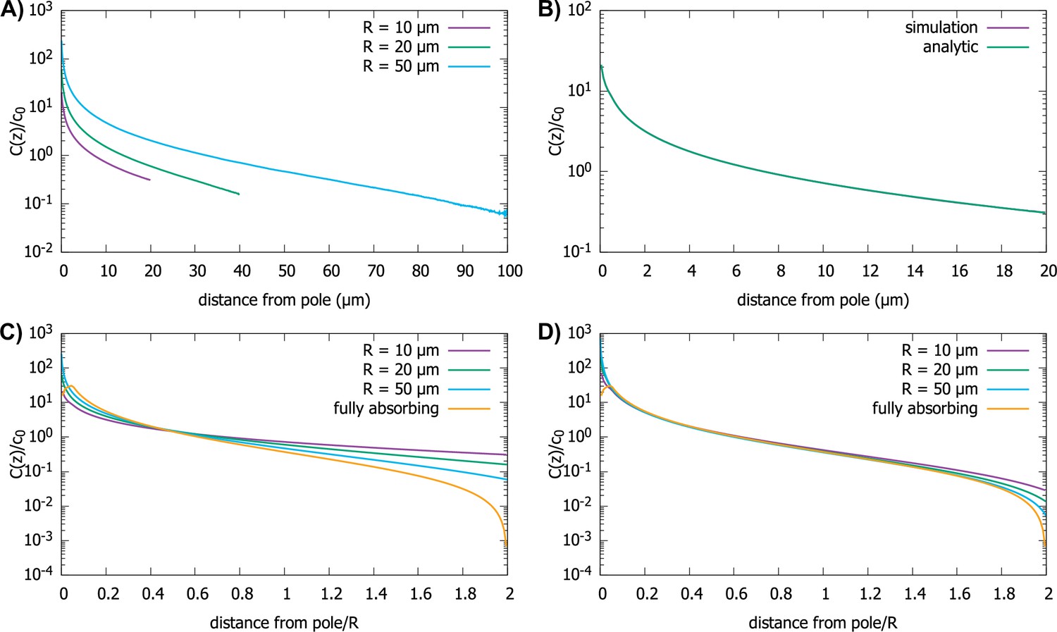
Figure 2

Download asset Open asset

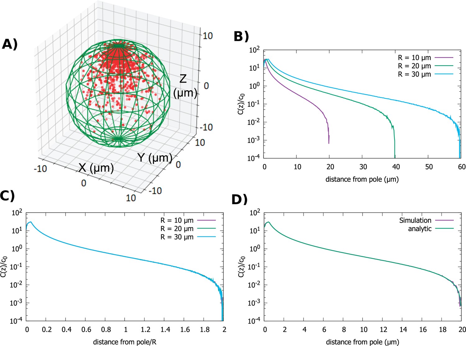
Concentration gradient in a spherical cell.

(A) Sample steady-state configuration obtained from the direct simulation of the polar transport model in a spherical cell with 1000 proteins (red). Direction of polar transport on the surface of the cell is toward the anterior pole, where the accumulation of proteins is observed. (B) Concentration of proteins along the polar, z-axis normalized by the average cytoplasmic concentration, for spherical cells of different radii. (C) Concentration profiles from B scaled by the cell radius. (D) Comparison between the steady-state solution of the polar transport equations (Equation 3), compared to the protein concentration obtained from simulations, for a spherical cell with radius $10 μ m$ . For all plots, the diffusion constant $D = 1 μ m^{2} / s$ and the transport speed along the cortex is $v = 1 μ m / s$ .

Figure 3

Download asset Open asset

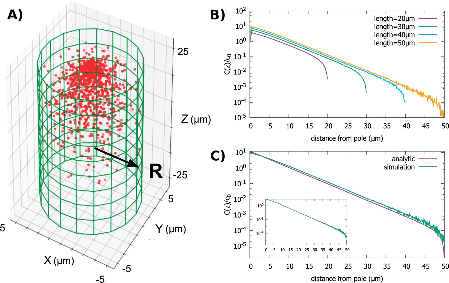
Protein gradient in a cylindrical cell.

(A) Configuration of the proteins obtained from simulation of the polar transport model with 1000 proteins (red circles). Directed transport on the surface of the cell is along positive z-direction. (B) Protein concentration along the z axis, normalized by the average cytoplasmic concentration, for cylindrical cells of different lengths and fixed radius, $R = 10 μ m$ . (C) Comparison between the steady-state solution of the polar transport equations and simulations. The analytic solution is an infinite series, and we compare the first term of this series to the results of simulations. The inset compares simulation results to the sum of the first 40 terms of the analytic solutions. For all plots, the diffusion constant $D = 1 μ m^{2} / s$ and the surface transport speed, $v = 1 μ m / s$ .

Figure 4

Download asset Open asset

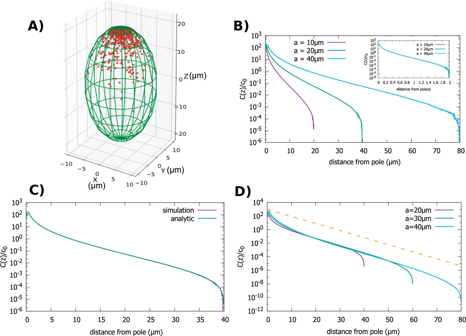
Concentration gradient in a spheroidal cell.

(A) Configuration of the proteins obtained from simulation of the polar transport model in a spheroidal cell of radius $R = 10 μ m$ and major axis $a = 20 μ m$ , and 1000 proteins. Direction of transport on the surface of the cell is along the positive z direction. (B) Protein concentration normalized by the average cytoplasmic concentration for spheroidal cells of different radii, with a fixed aspect ratio $\frac{a}{R} = 2$ . The inset shows concentration profiles where the distance from the pole is scaled by a. (C) Comparison between the analytic solution and simulations. (D) Concentration profiles for spheroids with the same minor axis ( $R = 10 μ m$ ) and a varying major axis ( $a$ ). The dashed line represents exponential decay with a decay constant $R / 2.4$ as we computed above, for the case of a cylindrical cell. For all plots, the diffusion constant $D = 1 μ m^{2} / s$ and the transport speed along the cortex is $v = 1 μ m / s$ .

Figure 5

Download asset Open asset

Effect of imperfect capture on the protein gradient.

(A) Protein concentration gradients (normalized by the average cytoplasmic concentration $c_{0}$ ) in spherical cells of different radii, computed by simulations of the polar transport model with 1000 particles. We use reactive boundary conditions with $k_{o n} = 0.1 μ$ m/s. (B) Comparison of the simulated protein gradient in a spherical cell, $R = 10 μ$ m, with reactive boundary conditions ( $k_{o n} = 0.1 μ$ m/s), to the analytical solution for the concentration profile (see Appendix C). (C) Analytic results for concentration gradients for different cell radii plotted against the distance from the pole scaled by the radius; $k_{o n} = 0.1 μ$ m/s. The scaling observed for fully absorbing boundary conditions (see Figure 2C) is absent. (D) Same as C, but now with $k_{o n} = 1 μ$ m/s. Scaling is approximately restored for most distances away from the pole. For all plots, the diffusion constant $D = 1 μ m^{2} / s$ and the transport speed along the cortex is $v = 1 μ m / s$ .

Figure 6

Download asset Open asset

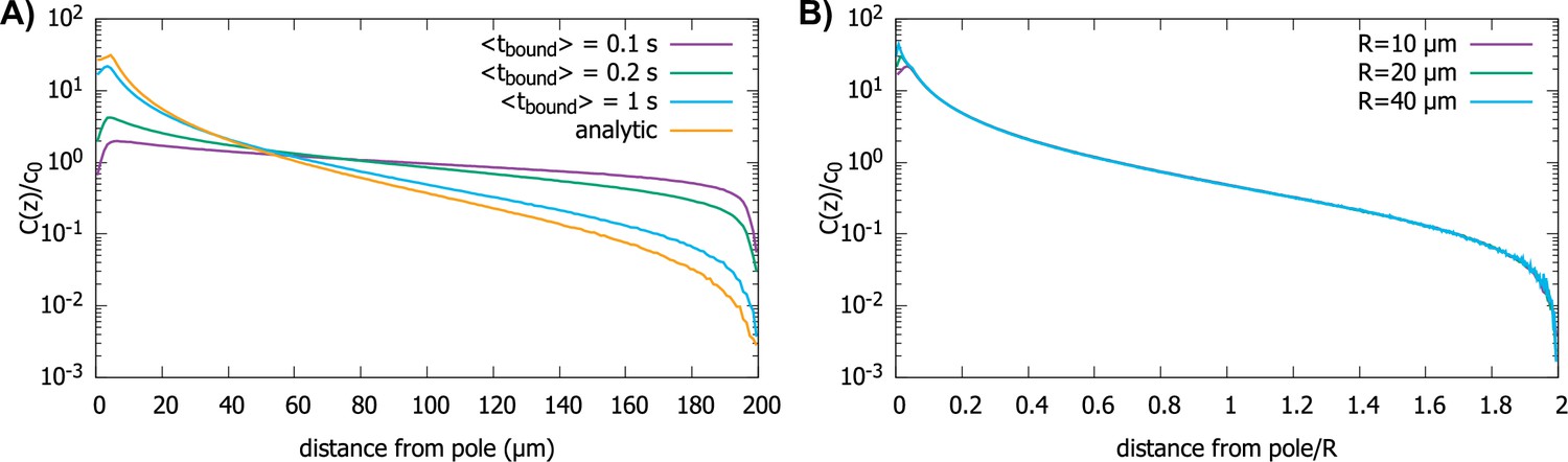
Effect of imperfect transport of proteins on the protein gradient.

(A) Concentration gradient obtained from simulation with 1000 proteins for various values of $⟨t_{b o u n d}⟩$ with a spherical cell of radius $R = 10 μ m$ . All other parameters are the same as in Figure 2. The analytic curve represents the gradient obtained from the polar transport model for a spherical cell. (B) Concentration gradients in a scaled coordinate for different values of $R$ with $⟨t_{b o u n d}⟩ = 1 s$ . For all plots, the diffusion constant $D = 1 μ m^{2} / s$ and the transport speed along the cortex is. $v = 1 μ m / s$ .

Appendix 1—figure 1

Download asset Open asset

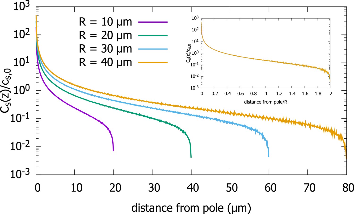
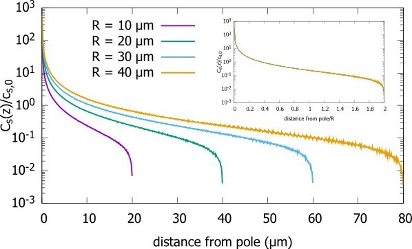
Surface concentration gradient for a spherical cell.

Concentration profiles on the surface of spherical cells of different radii, obtained from simulations of the polar transport model of gradient formations. Inset shows the same data, just with the distance from the pole scaled by the cell radius. Parameters used in the simulation: protein diffusion constant $D = 1 μ m^{2} / s$ , transport speed along the cortex $v = 1 μ m / s$ , and $ϵ / R = 0.05$ is the release point.

Author response image 1

Download asset Open asset

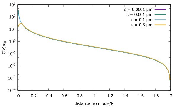
Concentration gradient for cells with the source at different distances from the pole (ε).

Concentration profiles with differing source points. We start very close to the pole and move further away. The radius of the sphere is $10 μ m$ , the diffusion constant $D = 1 μ m^{2} / s$ and the transport speed along the cortex is $v = 1 μ m / s$ .

Author response image 2

Download asset Open asset

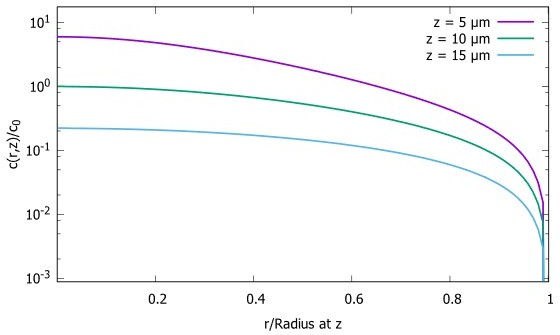
Concentration gradient in XY plane for a spherical cell.

Concentration Profiles in the XY plane for three different distances from the pole. The radius of the sphere is $10 μ m$ , the diffusion constant $D = 1 μ m^{2} / s$ and the transport speed along the cortex is $v = 1 μ m / s$ .

Author response image 3

Download asset Open asset

Surface concentration gradient for a spherical cell.

Additional files

Transparent reporting form: https://cdn.elifesciences.org/articles/71365/elife-71365-transrepform1-v2.pdf
Download elife-71365-transrepform1-v2.pdf

Download links

A two-part list of links to download the article, or parts of the article, in various formats.

Downloads (link to download the article as PDF)

Article PDF

Open citations (links to open the citations from this article in various online reference manager services)

Mendeley

Cite this article (links to download the citations from this article in formats compatible with various reference manager tools)

Arnab Datta
Sagnik Ghosh
Jane Kondev

(2022)

How to assemble a scale-invariant gradient

eLife 11:e71365.

https://doi.org/10.7554/eLife.71365

Sign up for email alerts

Privacy notice