Evolutionary footprints of a cold relic in a rapidly warming world
- Centre for Organismal Studies, University of Heidelberg, Germany
- Department of Ecology and Evolution, University of Lausanne, Switzerland
- Future Food Beacon and School of Life Sciences, the University of Nottingham, United Kingdom
Figures
Figure 1
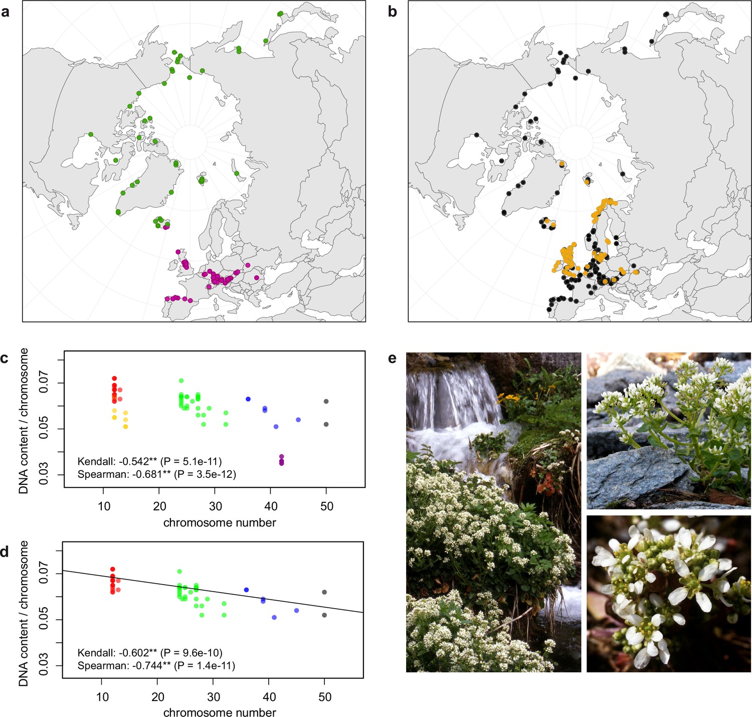
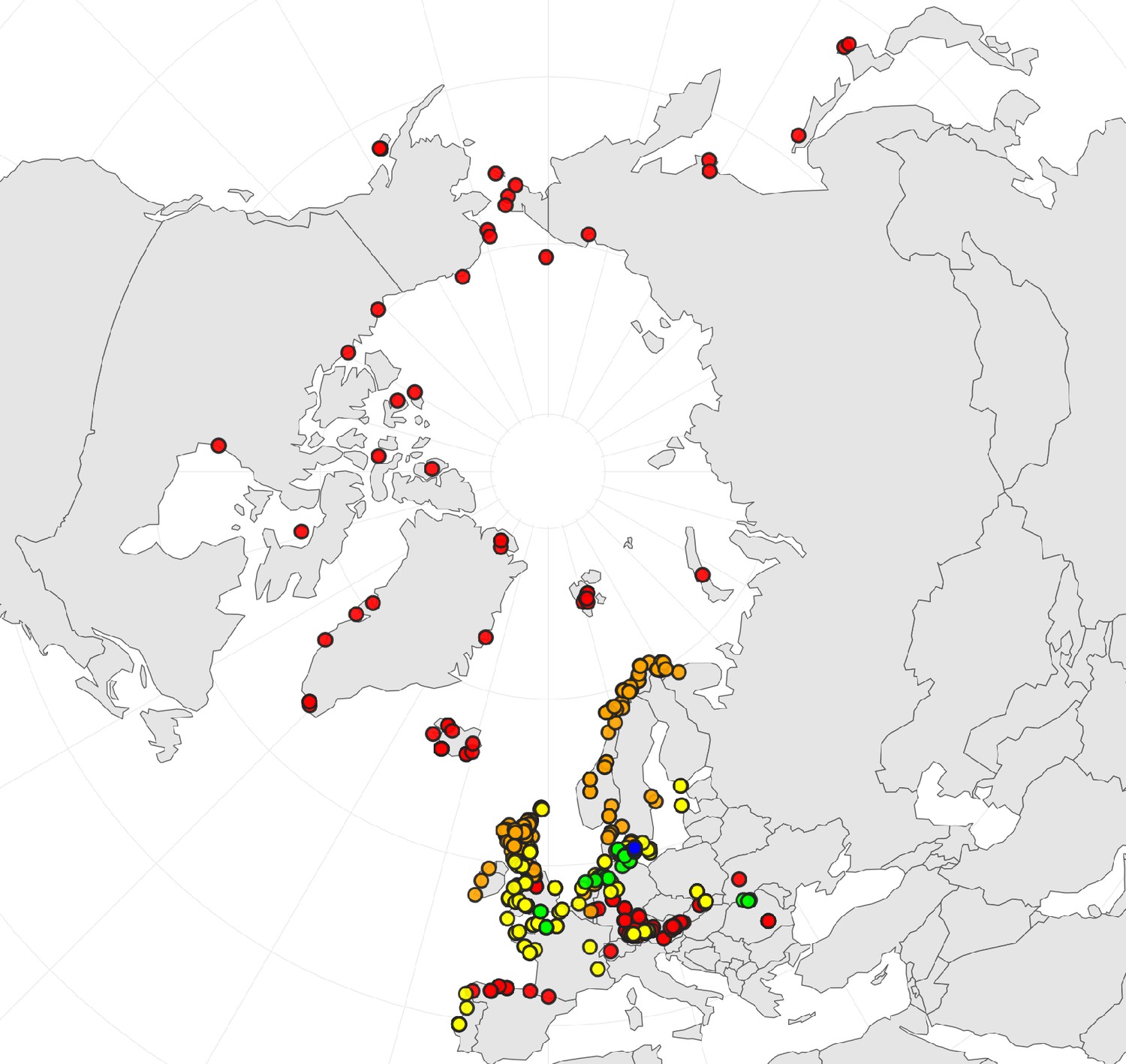
Distribution and cytogenomic flexibility of Cochlearia.
(a) Geographic distribution of chromosome counts for diploid Cochlearia accessions (n=169; Supplementary file 1 and Figure 1—source data 1), showing a clear separation of 2n=12 (European, green) and 2n=14 (Arctic, pink). (b) Geographic distribution of aneuploidies (orange, n=138) and euploidies (black, n=376) in diploid and polyploid Cochlearia (n=514; Figure 1—source data 2). (c) Measured DNA content per chromosome (given in picograms; Figure 1—source data 3) relative to respective total chromosome numbers (red [21 counts]: 2n=2x [non-Arctic], yellow [nine counts]: 2n=2x [Arctic], green [30 counts]: 2n=4x, blue [six counts]: 2n=6x [excluding C. danica], purple [10 counts]: 2n=6x [C. danica], dark grey [two counts]: 2n=8x) showing a significant decline of genome size per chromosome with increasing total chromosome numbers as revealed by Kendall and Spearman rank correlation analyses (78 individuals from 38 accessions representing 14 taxa analyzed in total) (data are not distributed normally and linear regression has not been performed). (d) Measured DNA content per chromosome (given in picograms; Figure 1—source data 4) relative to respective total chromosome numbers excluding Arctic diploids (yellow) and C. danica (purple) as putative outliers (59 individuals, 29 accessions, 11 taxa analyzed in total), showing a significant decline with increasing chromosome numbers via both rank correlation analyses and linear regression analysis (data are normally distributed and linear regression is significant with p=7.11e−10; R²=0.48; QQ-plot given with Appendix 1—figure 3). (e) Images of three Cochlearia species (left: C. pyrenaica [2n=2x=12], top right: C. tatrae [2n=6x=42], bottom right: C. anglica [2n=8x=48]) (data are normally distributed and linear regression is significant with p=7.11e−10; R²=0.48).
-
Figure 1—source data 1
Coordinates of diploid Cochlearia records in the survey of cytogenetic evolution.
- https://cdn.elifesciences.org/articles/71572/elife-71572-fig1-data1-v2.txt
-
Figure 1—source data 2
Coordinates of Cochlearia accessions with documented euploidies and aneuploidies in the survey of cytogenetic evolution.
- https://cdn.elifesciences.org/articles/71572/elife-71572-fig1-data2-v2.txt
-
Figure 1—source data 3
Measured DNA content per chromosome (given in picograms; full data set).
- https://cdn.elifesciences.org/articles/71572/elife-71572-fig1-data3-v2.txt
-
Figure 1—source data 4
Measured DNA content per chromosome (given in picograms; excluding Arctic diploids and C. danica as putative outliers).
- https://cdn.elifesciences.org/articles/71572/elife-71572-fig1-data4-v2.txt
Figure 2
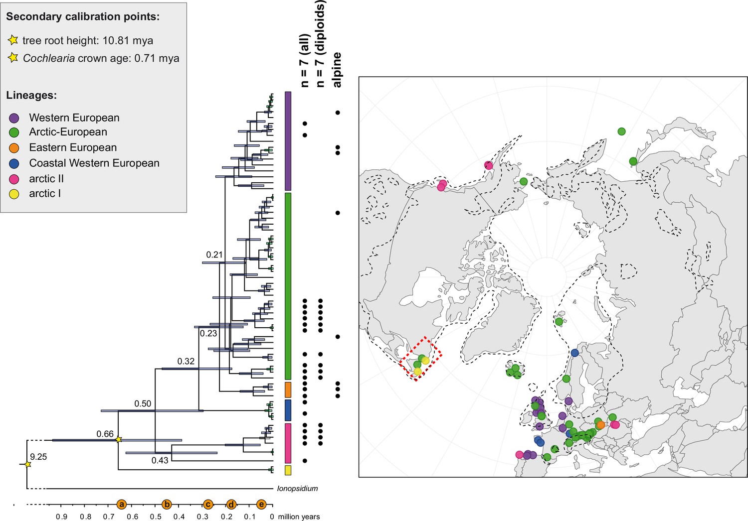
The maternal footprint of recurrent glacial speciation boosting.
BEAST chronogram (Figure 2—source data 1) based on complete plastid genome sequence data supplemented by a geographical distribution pattern of the six main phylogenetic lineages (displayed as colored bars next to the tree; dots in the map are colored accordingly; Figure 2—source data 2). The Ionopsidium outgroup lineage is collapsed and condensed. The tree topology is congruent to the topology as revealed from maximum likelihood (ML) analysis. The full BEAST chronogram and the ML tree (incl. bootstrap support values) are given in Appendix 1—figures 6, 9 and 10. Individuals with a base chromosome number of n=7 (shown for all ploidy levels and diploids only) and accessions with an alpine or subalpine habitat type are marked with black dots next to respective tips. Letters (a)–(e) as displayed on the timeline indicate high glacial periods: (a) 640 kya, end of Günz glacial; (b) 450 kya, beginning of Mindel glacial; (c) 250–300 kya, Mindel-Riss inter-glacial; (d) 150–200 kya, Riss glacial; (e) 30–80 kya, Würm glacial. The black dashed line indicates the extent of the Last Glacial Maximum (LGM ~21 kya; based on Ehlers and Gibbard, 2007). The red dashed rectangle highlights a region with evidence for ice-free areas during the Penultimate Glacial Period (~140 kya; based on Colleoni et al., 2016).
-
Figure 2—source data 1
BEAST chronogram in NEXUS format.
- https://cdn.elifesciences.org/articles/71572/elife-71572-fig2-data1-v2.txt
-
Figure 2—source data 2
Geographical distribution of phylogenetic lineages (plastid genome).
- https://cdn.elifesciences.org/articles/71572/elife-71572-fig2-data2-v2.txt
Figure 3
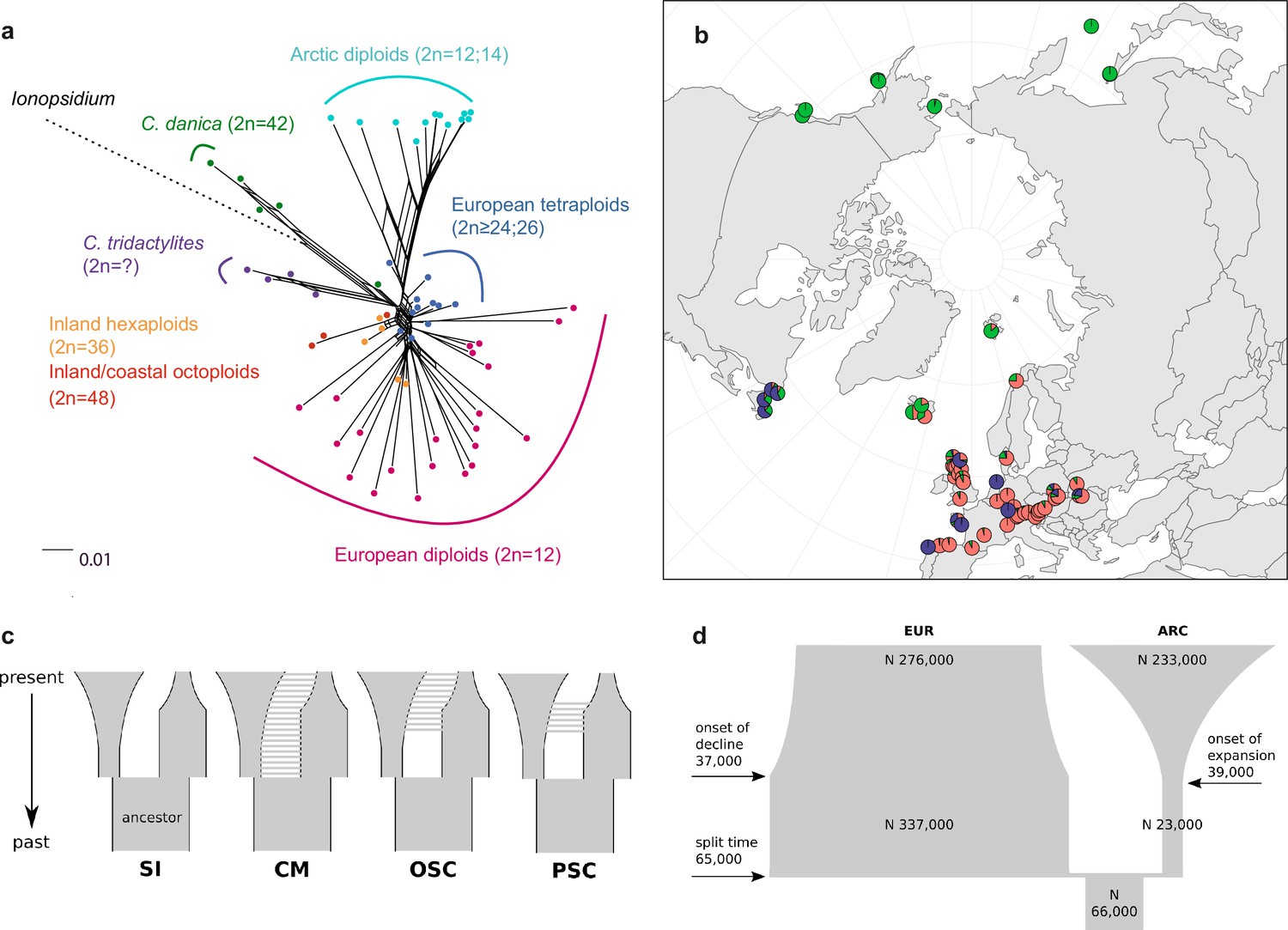
Demographic structure and history of the Cochlearia genus based on nuclear genome sequence data.
(a) SplitsTree analysis of 62 Cochlearia samples and Ionopsidium (outgroup) using the NeighborNet algorithm based on uncorrected p-distances (Figure 3—source data 1; network with tip labels is given with Appendix 1—figure 11). (b) Geographic distribution of 62 Cochlearia samples. Chart colors correspond to STRUCTURE results (62 Cochlearia samples; 400,071 variants) at K=3 (Figure 3—source data 2); green: Arctic gene pool, red: European gene pool, purple: C. danica-specific cluster (STRUCTURE result with tip labels given with Appendix 1—figure 15). (c) Coalescent models for diploid populations explored with Approximate Bayesian Computation (ABC). SI=strict isolation, CM=continuous migration from the population split to the present, OSC=ongoing secondary contact with gene flow starting after population split and continuing to the present, PSC=past secondary contact with gene flow starting after population split and stopping before the present. (d) Most likely demographic history of diploid EUR (2n=12) and ARC (2n=14) Cochlearia populations from coalescent modeling (based on 22 EUR individuals and 12 ARC individuals; 2140 SNPs at fourfold degenerate sites) and ABC of models without gene flow and upper bound of the population size (N) prior as 400,000 (Supplementary file 10). N is in number of diploid individuals, and time in number of generations ago.
-
Figure 3—source data 1
SplitsTree network in NEXUS format.
- https://cdn.elifesciences.org/articles/71572/elife-71572-fig3-data1-v2.txt
-
Figure 3—source data 2
STRUCTURE result at K=3 (georeferenced) and Delta K result (Evanno Method).
- https://cdn.elifesciences.org/articles/71572/elife-71572-fig3-data2-v2.txt
Figure 4
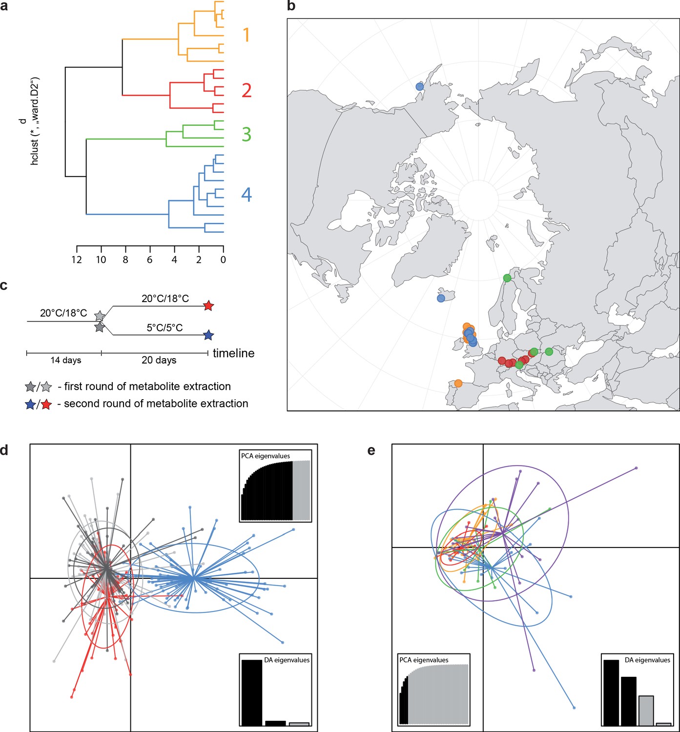
A common cold response indicated by metabolic profile clustering.
(a) Hierarchical cluster analysis of 28 Cochlearia accessions based on five temperature-related and four temperature/precipitation-related bioclimatic variables (WorldClim; given with Figure 4—source data 1) using Euclidian distances and the Ward’s method (Ward Jr JH, 1963; Murtagh and Legendre, 2014). Cluster 1: coastal accessions of polyploids from the northern UK; Cluster 2: European inland accessions (diploids and polyploids); Cluster 3: European accessions with Arctic/alpine habitat types (Norway, Carpathians, High Tatra Mountains, and Austrian Alps); Cluster 4: Arctic accessions (Iceland, Alaska) and alpine habitat types from the UK. (b) Geographical distribution of bioclimatic clusters as discovered via hierarchical cluster analysis (colors are representing clusters 1–4, see (a); Figure 4—source data 2). (c) Experimental setup of temperature treatment with a timeline for metabolite extractions. (d) DAPC based on all metabolic profiling measurements, grouped by treatment (colors are representing metabolite extractions as illustrated in c) (Figure 4—source data 3). (e) DAPC of metabolite measurements after cold treatment grouped by four bioclimatic clusters (colors as in (a) and (b)) and Ionopsidium (purple) (Figure 4—source data 1_SourceData4).
-
Figure 4—source data 1
9 WorldClim bioclimatic variables selected for hierarchical cluster analysis.
- https://cdn.elifesciences.org/articles/71572/elife-71572-fig4-data1-v2.txt
-
Figure 4—source data 2
Geographical distribution of bioclimatic clusters.
- https://cdn.elifesciences.org/articles/71572/elife-71572-fig4-data2-v2.txt
-
Figure 4—source data 3
DAPC result based on all metabolic profiling measurements, grouped by treatment.
- https://cdn.elifesciences.org/articles/71572/elife-71572-fig4-data3-v2.txt
Appendix 1—figure 1

Illustration of previous evolutionary hypotheses.
A summary of hypotheses regarding the evolution of the genus Cochlearia combined with information on ploidy levels and ecology. The latter is given as a combination of (a) species distribution, and (b) substrate specificity.
Appendix 1—figure 2
Geographic distribution of ploidy levels in Cochlearia (n=564) as revealed via a review of published and own chromosome counts (Supplementary file 2 and Appendix 1—figure 2—source data 1).
Diploids are colored in red, tetraploids in orange, hexaploids in yellow, octoploids in green, and dodecaploids in blue.
-
Appendix 1—figure 2—source data 1
Geographical distribution of ploidy levels in documented Cochlearia accessions.
- https://cdn.elifesciences.org/articles/71572/elife-71572-app1-fig2-data1-v2.zip
Appendix 1—figure 3
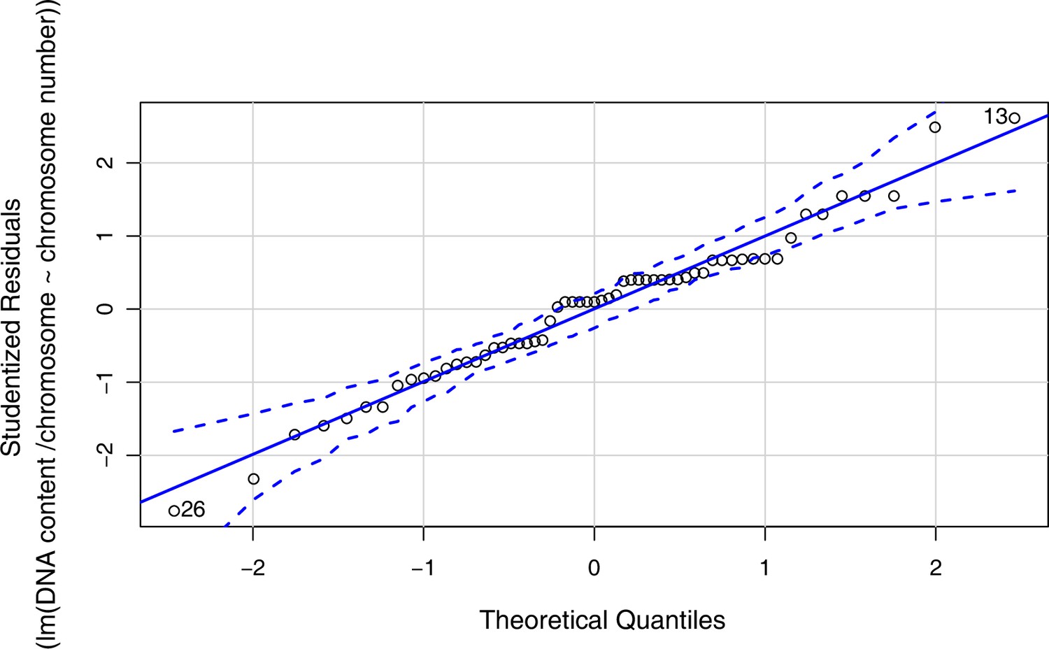
Quantile-Quantile Plot generated using the qqPlot() function in R version 4.0.3 (confidence level for point-wise envelope set to 0.99) as a visual check used to assess data normality for linear regression analysis shown in Figure 1d (data given with Figure 1—source data 4).
Appendix 1—figure 4

Genome size increase with increasing ploidy levels.
Measured 2C value (given in picograms) relative to respective total chromosome numbers. (a) Full data set (red [21 counts]: 2n=2x (non-Arctic), yellow [nine counts] 2n=2x [Arctic], green [30 counts]: 2n=4x, blue [six counts]: 2n=6x [excluding C. danica], purple [10 counts]: 2n=6x [C. danica], dark grey [two counts]: 2n=8x) showing a significant increase of genome size with increasing total chromosome numbers as revealed by Kendall and Spearman rank correlation analyses (78 individuals from 38 accessions representing 14 taxa analyzed in total; Appendix 1—figure 4—source data 1). (B), Data set excluding short-lived Arctic diploids (yellow) and annual C. danica (purple) as putative outliers, showing a significant genome size increase with increasing chromosome numbers as revealed by Kendall and Spearman rank correlation analyses (59 individuals, 29 accessions, 11 taxa analyzed in total; Appendix 1—figure 4—source data 2).
-
Appendix 1—figure 4—source data 1
Measured 2C values (in picograms) of all analyzed Cochlearia samples as used for rank correlation analyses (2C value / total chromosome number).
- https://cdn.elifesciences.org/articles/71572/elife-71572-app1-fig4-data1-v2.zip
-
Appendix 1—figure 4—source data 2
Measured 2C values (in picograms) of Cochlearia samples excluding short-lived arctic diploids and the annual C. danica as putative outlier samples as used for rank correlation analyses (2C value / total chromosome number).
- https://cdn.elifesciences.org/articles/71572/elife-71572-app1-fig4-data2-v2.zip
Appendix 1—figure 5
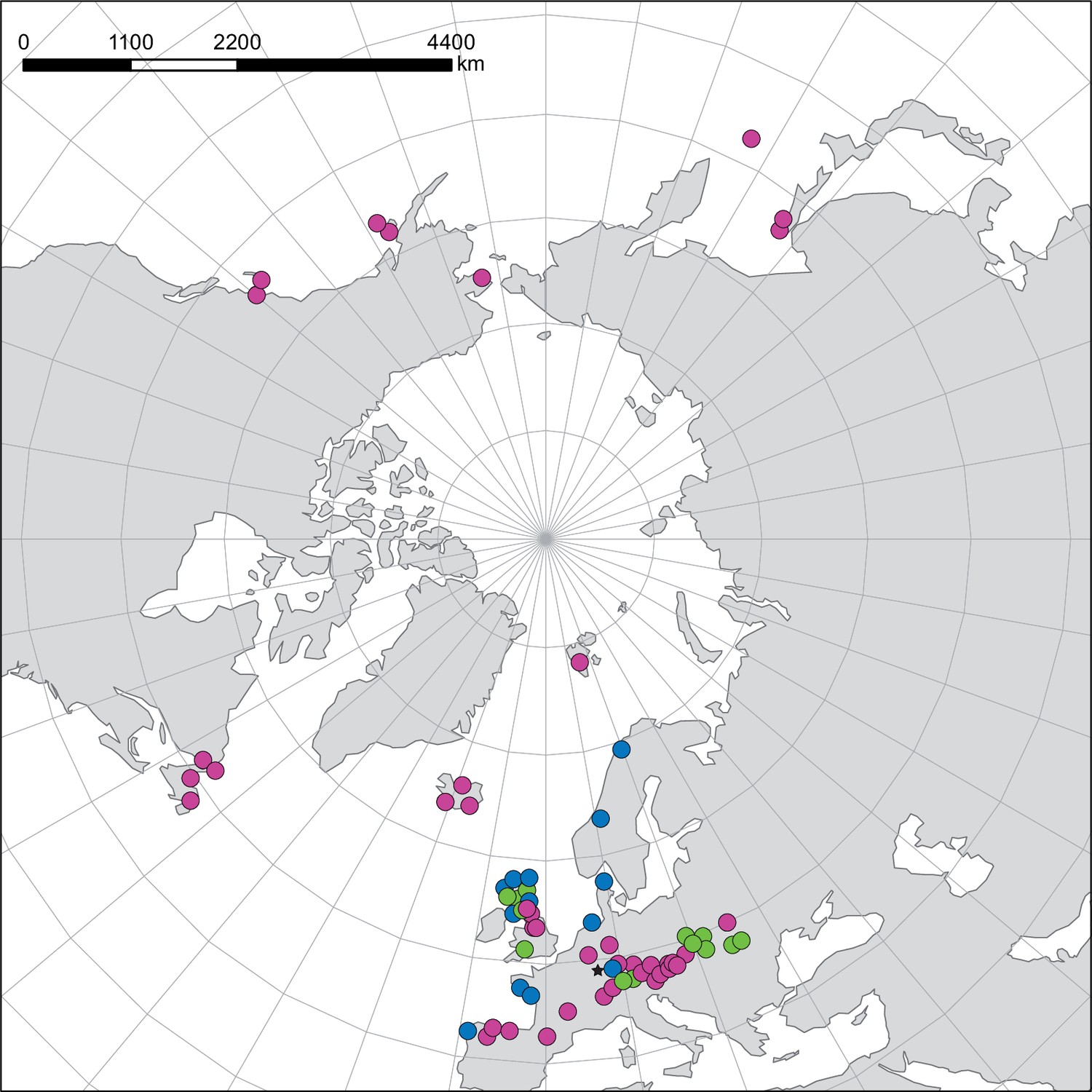
NGS samples—geographical distribution and ploidy levels/ecotypes.
Geographical distribution of Cochlearia NGS samples. Colors indicate different ploidy levels/ecotypes. Diploid samples are shown in pink, polyploid inland samples in green, and polyploid coastal samples in blue. The asterisk marks an inland sample of C. danica which is a coastal species rapidly dispersed inland along highways.
Appendix 1—figure 6
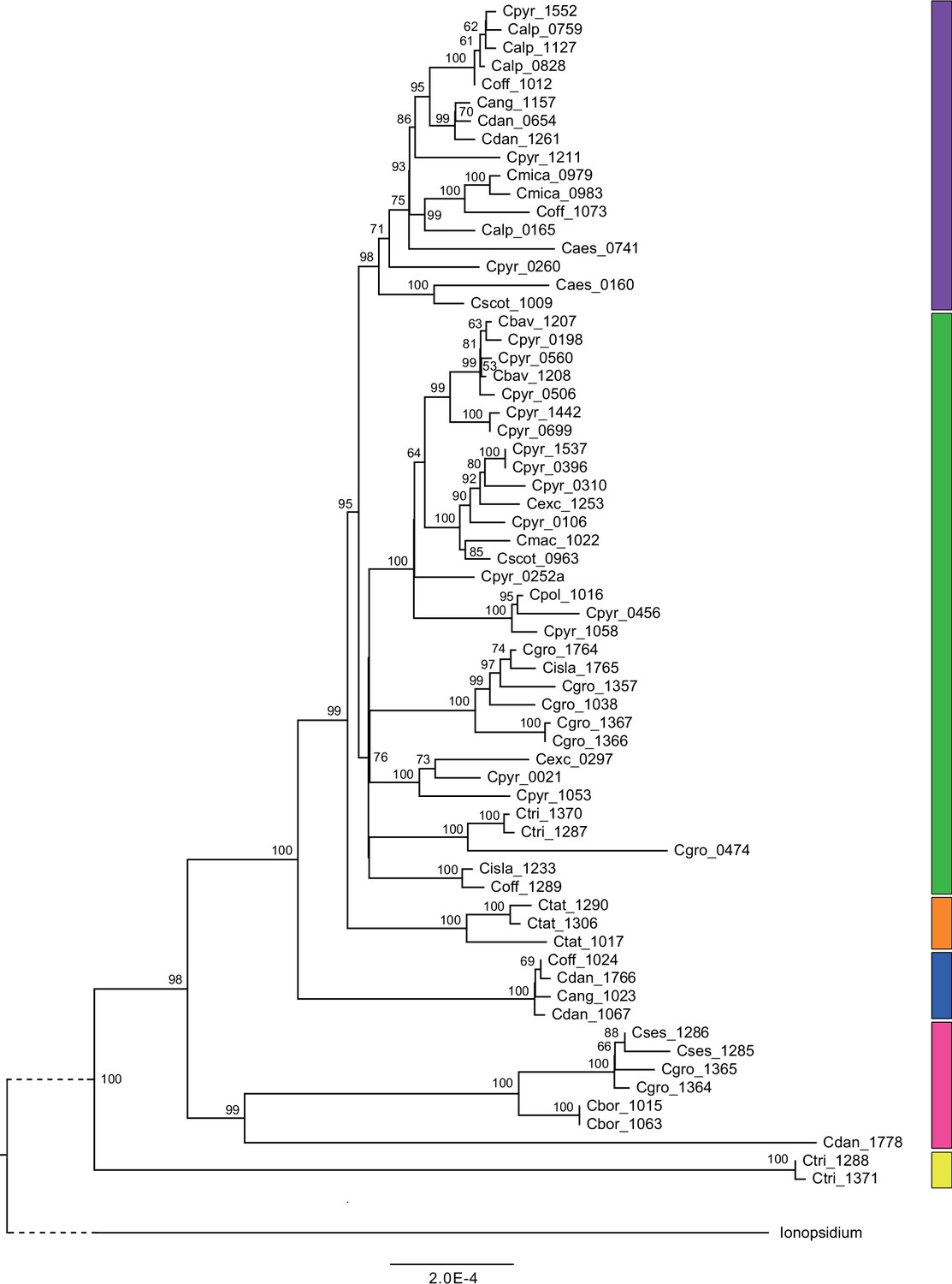
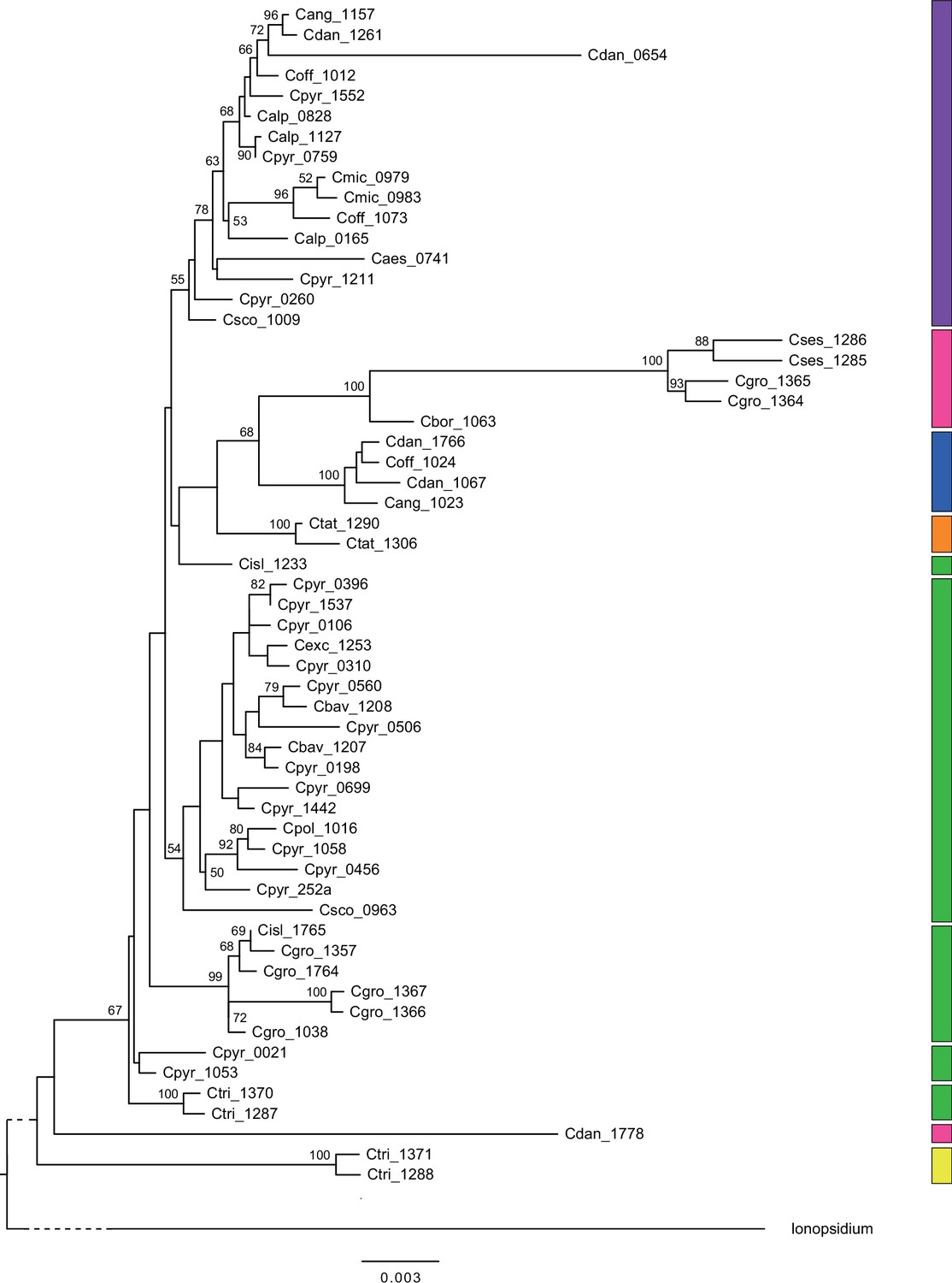
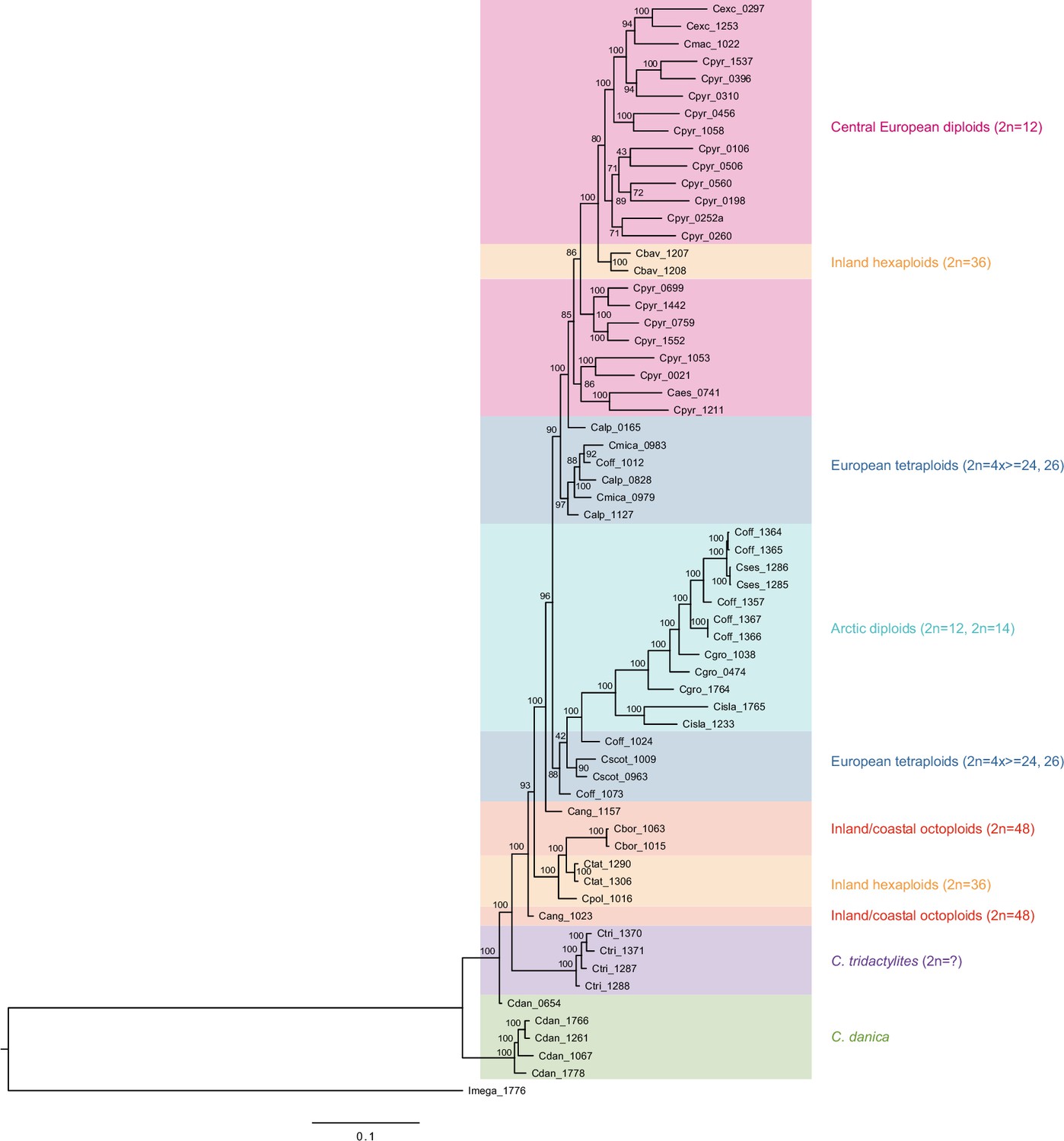
Plastid maximum likelihood (ML) phylogeny.
ML phylogram based on complete chloroplast genomes from the tribe Cochlearieae generated with RAxML (Appendix 1—figure 6—source data 1). Bootstrap support (1000 replicates) above 50% is shown near the respective nodes. For illustration purpose, the Ionopsidium outgroup lineage is collapsed and condensed. Evolutionary lineages within Cochlearia are displayed as colored bars (corresponding to Figure 2). Taxa included in evolutionary lineages: yellow lineage: C. tridactylites; pink lineage: C. danica, C. borzaeana, C. groenlandica, C. sessilifolia; blue lineage: C. danica, ‘C. anglica’ (or C. hollandica), C. officinalis; orange lineage: C. tatrae; green lineage: C. officinalis, C. islandica, C. groenlandica, C. tridactylites, C. pyrenaica, C. excelsa, C. polonica, C. scotica, C. macrorrhiza, C. bavarica; purple lineage: C. scotica, C. aestuaria, C. pyrenaica, C. alpina, C. officinalis, C. micacea, C. danica, ‘C. anglica/hollandica.’
-
Appendix 1—figure 6—source data 1
Best-scoring ML tree based on (nearly) complete plastid genomes and generated in RAxML with 1000 rapid bootstraps.
- https://cdn.elifesciences.org/articles/71572/elife-71572-app1-fig6-data1-v2.zip
Appendix 1—figure 7
Mitochondrial maximum likelihood (ML) phylogeny.
ML tree (Appendix 1—figure 7—source data 1) based on 58 partial mitochondrial genomes of genus Cochlearia and one outgroup sample of genus Ionopsidium (Ionopsidium megalospermum, sample-ID: Imega_1776). The latter is shown condensed for a better illustration of Cochlearia samples. Bootstrap support (1000 replicates) above 50% is shown near the respective nodes and colored blocks to the right correspond to respective chloroplast lineages as displayed in Figure 2.
-
Appendix 1—figure 7—source data 1
Best-scoring ML tree based on partial mitochondrial genomes and generated in RAxML with 1000 rapid bootstraps.
- https://cdn.elifesciences.org/articles/71572/elife-71572-app1-fig7-data1-v2.zip
Appendix 1—figure 8
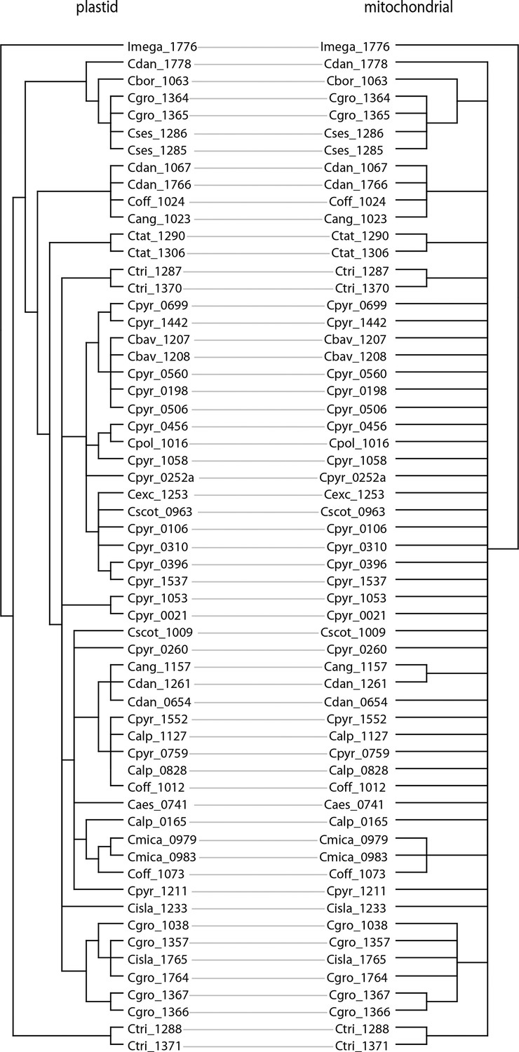
Tanglegram of plastid and mitochondrial phylogenies.
The tanglegram was generated with dendroscope (Huson and Scornavacca, 2012) and branches with bootstrap support below 95% were collapsed prior to the analysis (Appendix 1—figure 8—source data 1).
-
Appendix 1—figure 8—source data 1
Tanglegram nexus-file (plastome versus mitochondrial sequence data).
- https://cdn.elifesciences.org/articles/71572/elife-71572-app1-fig8-data1-v2.zip
Appendix 1—figure 9
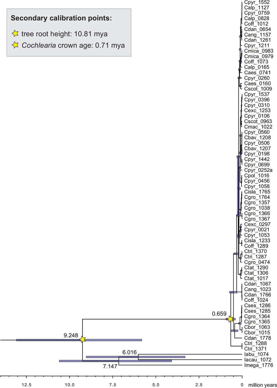
Cochlearieae maternal timeline.
Cochlearieae BEAST chronogram based on whole chloroplast genome sequence data (Figure 2—source data 1). Secondary calibration points are indicated accordingly. Divergence times for the Ionopsidium/Cochlearia split, the genus Ionopsidium, and the Cochlearia crown age are indicated with 95% confidence intervals. Divergence time estimates within genus Cochlearia are given with Appendix 1—figure 10.
Appendix 1—figure 10

Cochlearia divergence time estimates.
BEAST chronogram based on complete chloroplast genomes (Figure 2—source data 1). For illustration purpose, the Ionopsidium outgroup lineage is collapsed and condensed. The two secondary calibration points are indicated accordingly and divergence times older than 0.02 mya age are indicated with 95% confidence intervals. Green node bars indicate divergence times younger than 0.02 mya. Major evolutionary lineages within Cochlearia are displayed as colored bars (corresponding to Figure 3). Taxa included in evolutionary lineages: yellow lineage: C. tridactylites; pink lineage: C. danica, C. borzaeana, C. groenlandica, C. sessilifolia; blue lineage: C. danica, ‘C. anglica/C. hollandica,’ C. officinalis; orange lineage: C. tatrae; green lineage: C. officinalis, C. islandica, C. groenlandica, C. tridactylites, C. pyrenaica, C. excelsa, C. polonica, C. scotica, C. macrorrhiza, C. bavarica; purple lineage: C. scotica, C. aestuaria, C. pyrenaica, C. alpina, C. officinalis, C. micacea, C. danica, ‘C. anglica/hollandica.’ Letters displayed on the timeline indicate high glacial periods as follows: (a) 640 ky, end of Günz glacial; (b) 450 ky, begin of Mindel glacial; (c) 250–300 ky, Mindel-Riss inter-glacial; (d) 150–200 ky, Riss glacial; (e) 30–80 ky, Würm glacial.
Appendix 1—figure 11
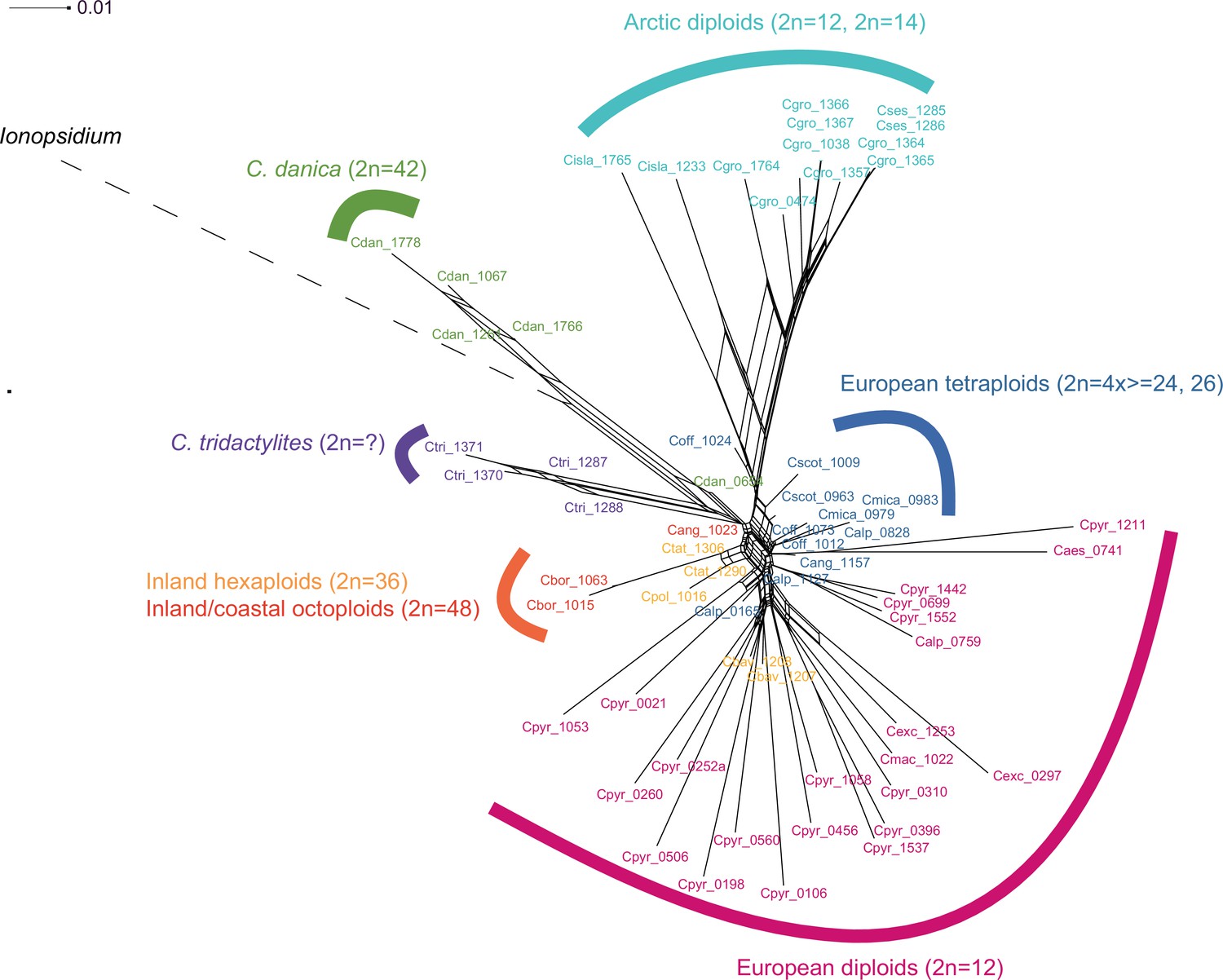
Detailed SplitsTree output.
Result of a SplitsTree analysis of Cochlearia samples and Ionopsidium (outgroup) using the NeighborNet algorithm based on uncorrected p-distances (Figure 3—source data 1). For illustration purpose, the Ionopsidium branch is condensed.
Appendix 1—figure 12
Maximum likelihood tree based on transcriptome-wide nuclear SNPs.
The tree was generated with RAxML and the analysis (based on 298,978 variant sites) was performed with an ascertainment bias correction in order to account for sampling only variable sites (Appendix 1—figure 12—source data 1). Bootstrap support (1000 replicates) is shown near the respective nodes and coloring of sample groups corresponds to respective colors in the SplitsTree output as visualized in Figure 3a.
-
Appendix 1—figure 12—source data 1
Best-scoring ML tree based on transcriptome-wide nuclear SNPs (298,978 variant sites) and generated in RAxML with an ascertainment bias correction and 1000 rapid bootstraps.
- https://cdn.elifesciences.org/articles/71572/elife-71572-app1-fig12-data1-v2.zip
Appendix 1—figure 13
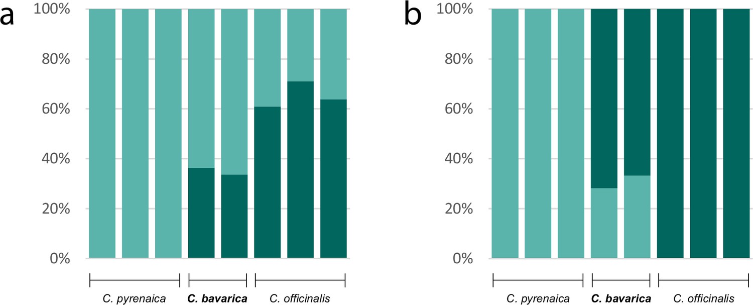
Genetic assignment analyses investigating the allopolyploid origin of the hexaploid species Cochlearia bavarica (2n=6x=36).
Results of two STRUCTURE analyses based on nuclear transcriptome data (coding and non-coding; 103,874 variants) of two C. bavarica samples and samples from putative parental species C. pyrenaica (2n=2x=12) and C. officinalis (2n=4x=24). The analyses were performed under the uncorrelated (a; Appendix1-file13_SourceData1) and the correlated (b; Appendix1-file13_SourceData2) allele frequency models respectively, both assuming K=2.
-
Appendix 1—figure 13—source data 1
STRUCTURE result C. bavarica at K=2 (uncorrelated allele frequency model).
- https://cdn.elifesciences.org/articles/71572/elife-71572-app1-fig13-data1-v2.zip
-
Appendix 1—figure 13—source data 2
STRUCTURE result C. bavarica at K=2 (correlated allele frequency model).
- https://cdn.elifesciences.org/articles/71572/elife-71572-app1-fig13-data2-v2.zip
Appendix 1—figure 14
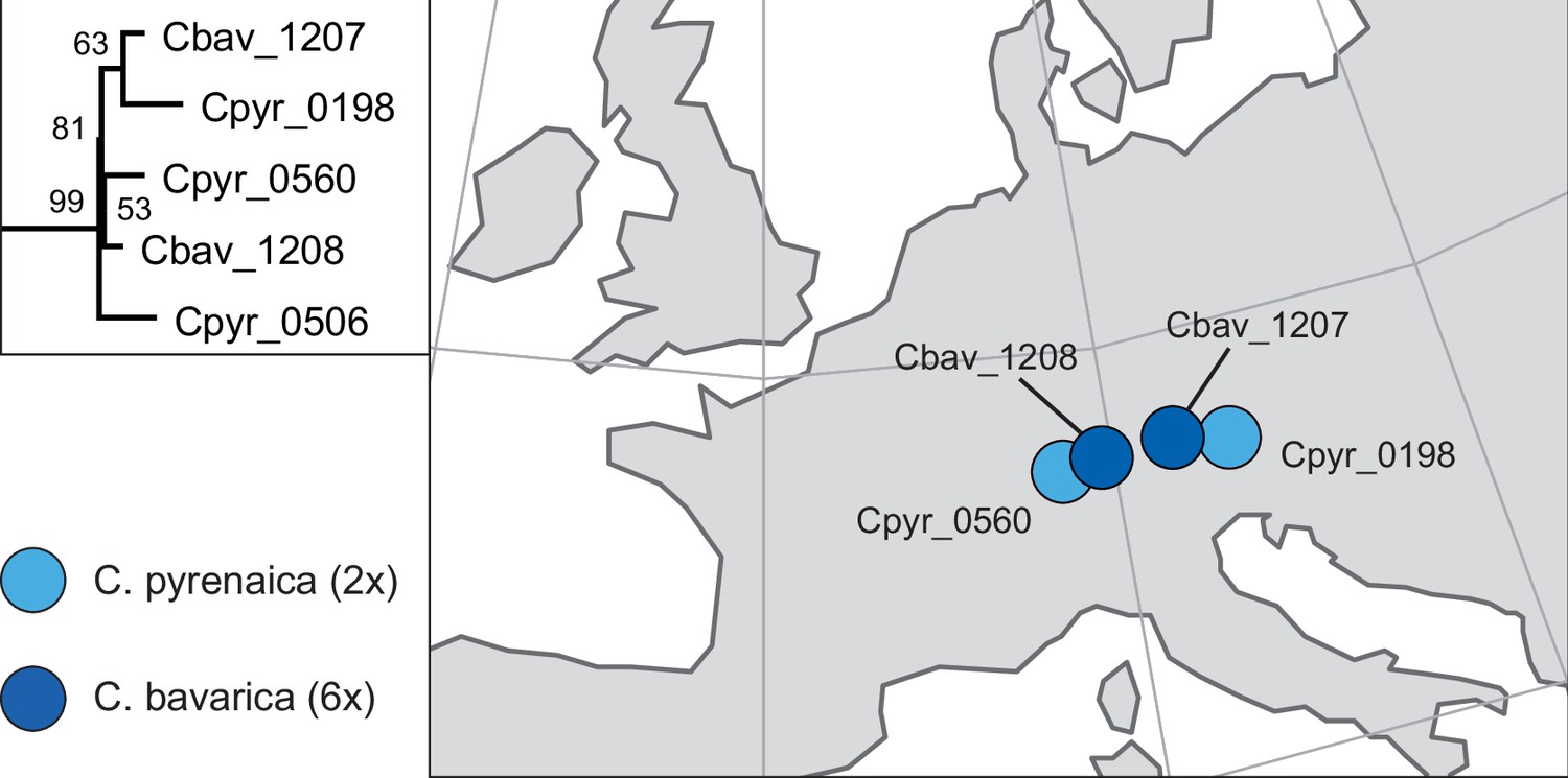
Phylogenetic placement and geographical occurrence of hexaploid Cochlearia bavarica.
Geographically close populations of C. pyrenaica as putative maternal plants in past allopolyploidization processes of C. bavarica as revealed from the maximum likelihood plastid phylogeny (see Appendix 1—figure 6). Results are consistent with earlier population-based analyses using isozyme studies from multiple populations (Koch, 2002).
Appendix 1—figure 15
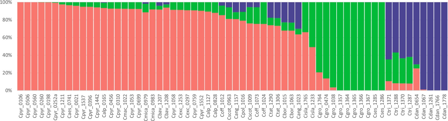
Genetic assignment analysis of the genus Cochlearia (all samples).
Result of a STUCTURE analysis for all 62 Cochlearia samples assuming K=3 (correlated allele frequencies) based on 101,386 SNPs detected within 1,425,819 callable loci throughout the transcriptome (coding and non-coding). Colors correspond to the geographical representation as shown in Figure 3, Figure 3—source data 2. Every bar represents one individual and sample names are given below respective bars.
Appendix 1—figure 16

Optimal number of migration edges for TreeMix analysis.
The optimal value of m (migration edges, x-axis) was assessed according to the Evanno method (deltaM, y-axis) across 10 replicates of each m from m=1 to m=10.
Appendix 1—figure 17

TreeMix residuals m=0.
Residual plot of a TreeMix analysis with m = 0. Individuals (populations) that are not well-modeled can be identified by residuals deviating from zero with positive residuals indicating an underestimate of the observed covariance. Here, the fit of the model might be improved by additional migration edges.
Appendix 1—figure 18
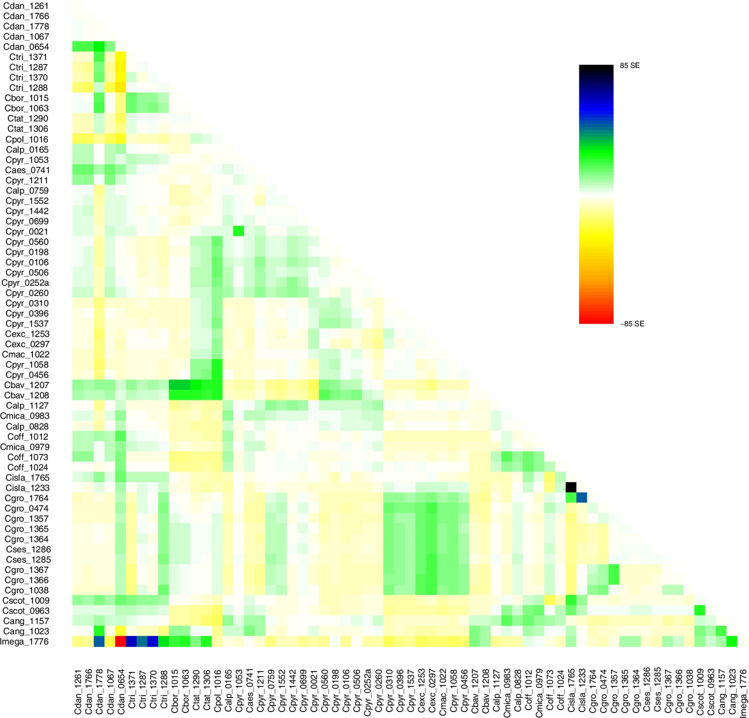
TreeMix residuals m=1.
Residual plot of a TreeMix analysis with m=1 (best m, Evanno method; Evanno et al., 2005). Individuals (populations) that are not well-modeled can be identified by residuals deviating from zero with positive residuals indicating an underestimate of the observed covariance. Here, the fit of the model might be improved by additional migration edges.
Appendix 1—figure 19
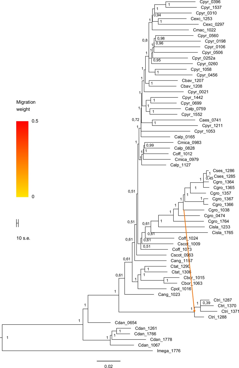
TreeMix bootstrapped tree with migration edge (m=1).
The maximum likelihood consensus tree (_SourceData1)Appendix 1—figure 19—source data 1 was generated with TreeMix (Pickrell and Pritchard, 2012) with one migration/admixture event (best m, Evanno method; Appendix 1—figure 16). TreeMix analysis indicates that migration occurred from Arctic C. groenlandica (2n=14) to Eastern Canadian C. tridactylites (2n=?). Migration arrow is colored by migration weight and indicates the direction of gene flow. The consensus tree was inferred from 100 bootstrap replicates using SumTrees (Sukumaran and Holder, 2010).
-
Appendix 1—figure 19—source data 1
Bootstrapped (100 bootstrap replicates) maximum likelihood consensus tree generated with TreeMix with one migration/admixture event.
- https://cdn.elifesciences.org/articles/71572/elife-71572-app1-fig19-data1-v2.zip
Appendix 1—figure 20
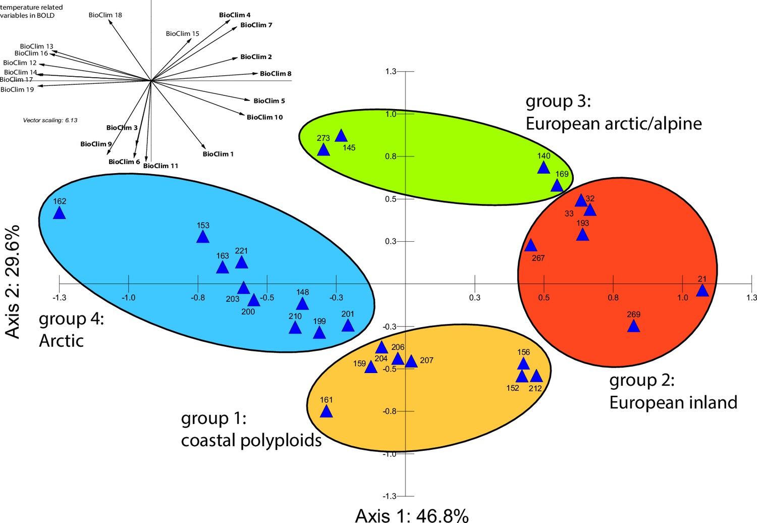
Principal component analysis (PCA) based on all 19 bioclimatic variables.
PCA result based on all 19 WorldClim bioclimatic variables for 28 Cochlearia accessions (Appendix 1—figure 20—source data 1); biplot of the first two axes explaining 76.4% of the total variance. Group colors correspond to bioclimatic clusters (Figure 4) as also defined by hierarchical cluster analysis.
-
Appendix 1—figure 20—source data 1
19 WorldClim bioclimatic variables for 28 Cochlearia accessions.
- https://cdn.elifesciences.org/articles/71572/elife-71572-app1-fig20-data1-v2.zip
Appendix 1—figure 21
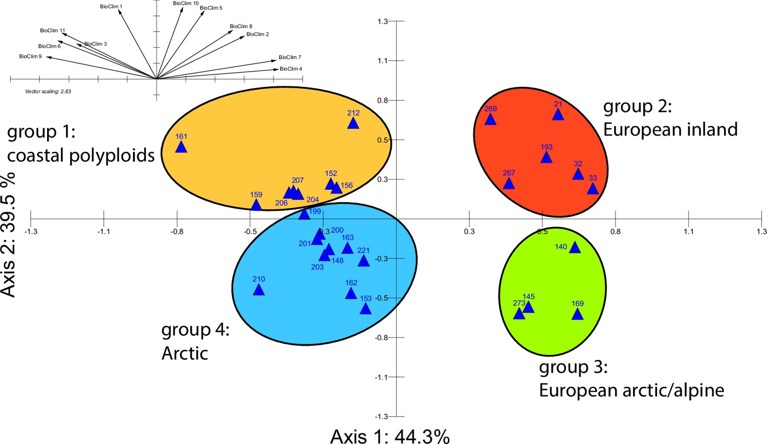
Principal component analysis (PCA) based on bioclimatic variables.
PCA result based on WorldClim bioclimatic variables 1–11 (temperature-related) for 28 Cochlearia accessions (Appendix 1—figure 21—source data 1); biplot of the first two axes explaining 83.8% of the total variance. Group colors correspond to bioclimatic clusters (Figure 4) as also defined by hierarchical cluster analysis.
-
Appendix 1—figure 21—source data 1
11 WorldClim bioclimatic variables for 28 Cochlearia accessions.
- https://cdn.elifesciences.org/articles/71572/elife-71572-app1-fig21-data1-v2.zip
Appendix 1—figure 22
Alkaloid relative levels (normalized to the ribitol internal standard) under control/cold conditions.
Boxplots showing means of normalized levels to the ribitol internal standard (y-axis) of analyzed alkaloids in plants from four bioclimatic Cochlearia clusters (x-axis: 1–4; see Figure 4a) and (b) and Ionopsidium (x-axis: 5) as measured by gas chromatography-mass spectrometry after growing under control (18°C/20 °C, red) or cold (5°C, blue) conditions for 20 days. No significant differences between the two treatments within each cluster were revealed via one-way ANOVA (Appendix 1—figure 22—source data 1).
-
Appendix 1—figure 22—source data 1
Detailed summary output of one-way ANOVAs for all metabolites for bioclimatic clusters (1–4) and Ionopsidium (5).
- https://cdn.elifesciences.org/articles/71572/elife-71572-app1-fig22-data1-v2.zip
Appendix 1—figure 23
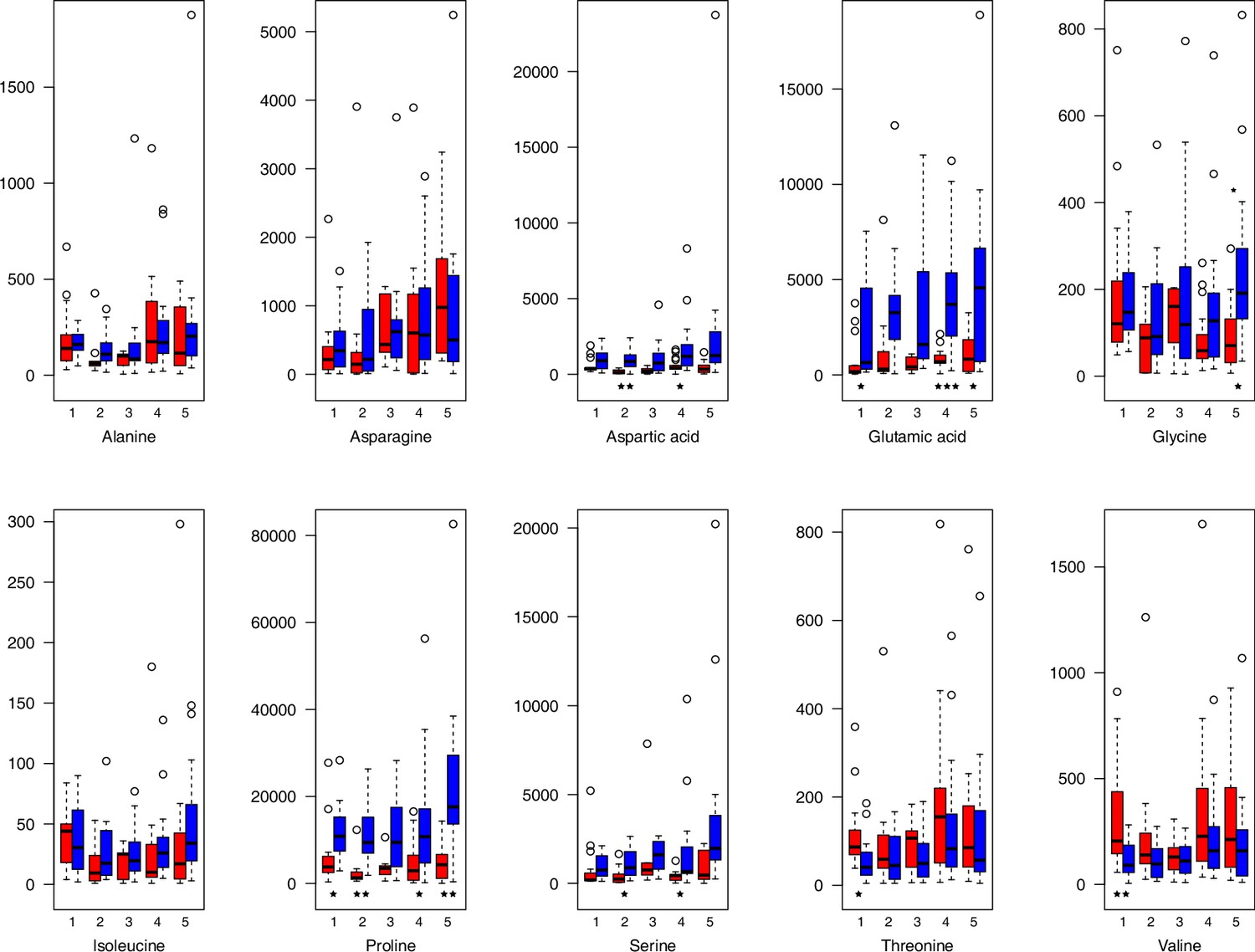
Amino acid relative levels (normalized to the ribitol internal standard) under control/cold conditions.
Boxplots showing means of normalized levels to the ribitol internal standard (y-axis) of analyzed amino acids in plants from four bioclimatic Cochlearia clusters (x-axis: 1–4; see Figure 4a and b) and Ionopsidium (x-axis: 5) as measured by gas chromatography-mass spectrometry after growing under control (18°C/20°C, red) or cold (5°C, blue) conditions for 20 days. Significant differences between the two treatments within each cluster as revealed via one-way ANOVA are indicated by asterisks (*p≤0.05; **p≤0.02; ***p≤0.001; Appendix 1—figure 22—source data 1).
Appendix 1—figure 24
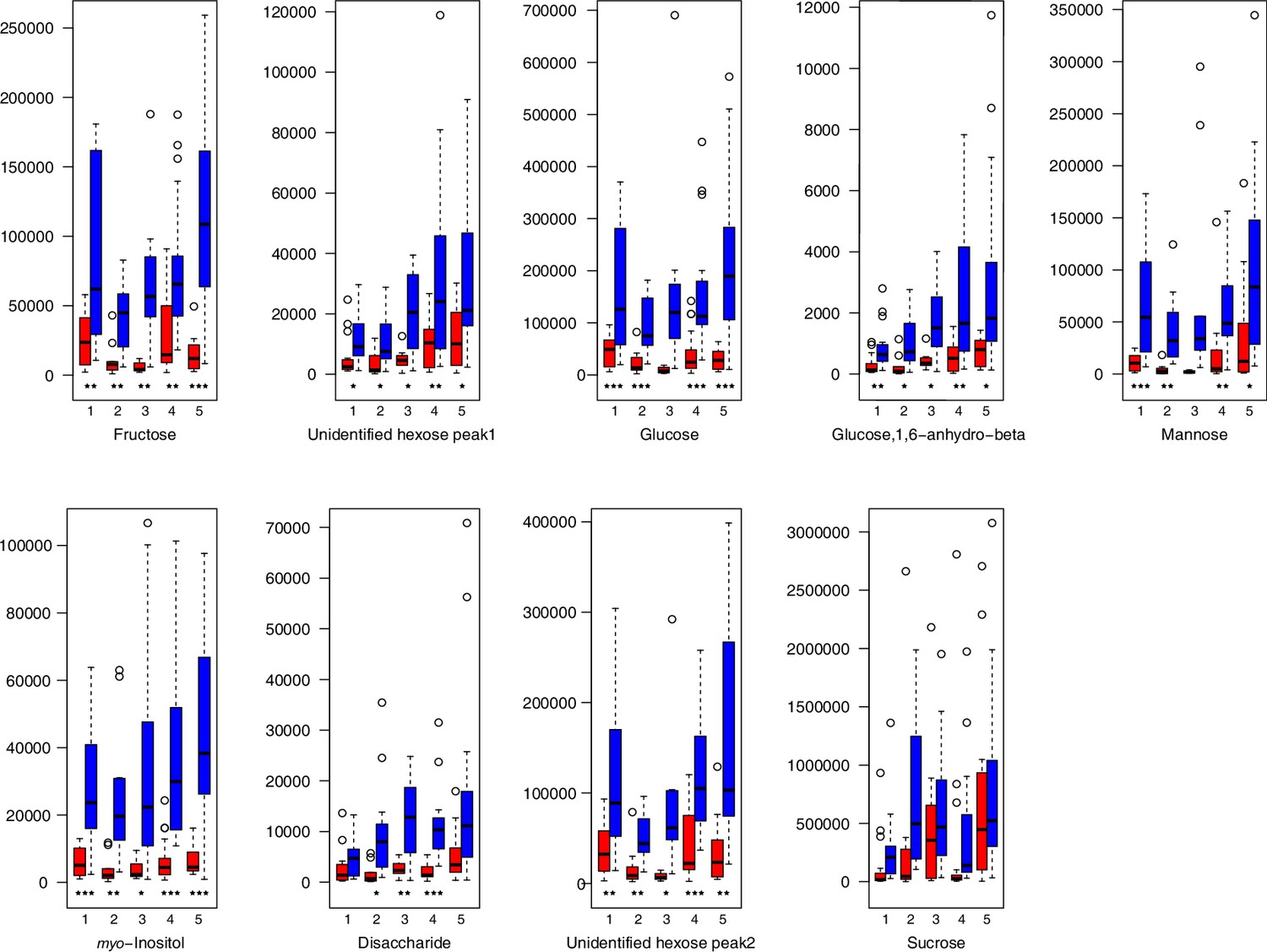
Carbohydrate relative levels (normalized to the ribitol internal standard) under control/cold conditions.
Boxplots showing means of normalized levels to the ribitol internal standard (y-axis) of analyzed carbohydrates in plants from four bioclimatic Cochlearia clusters (x-axis: 1–4; see Figure 4a and b) and Ionopsidium (x-axis: 5) as measured by gas chromatography-mass spectrometry after growing under control (18°C/20°C, red) or cold (5°C, blue) conditions for 20 days. Significant differences between the two treatments within each cluster as revealed via one-way ANOVA are indicated by asterisks (*p≤0.05; **p≤0.02; ***p≤0.001; Appendix 1—figure 22—source data 1).
Appendix 1—figure 25
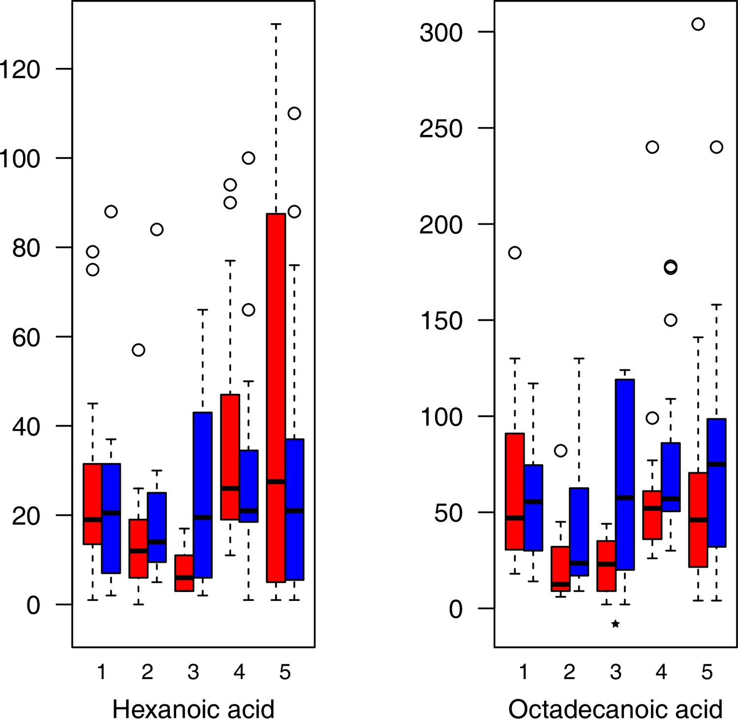
Fatty acid relative levels (normalized to the ribitol internal standard) under control/cold conditions.
Boxplots showing means of normalized levels to the ribitol internal standard (y-axis) of analyzed fatty acids in plants from four bioclimatic Cochlearia clusters (x-axis: 1–4; see Figure 4a and b) and Ionopsidium (x-axis: 5) as measured by gas chromatography-mass spectrometry after growing under control (18°C/20°C, red) or cold (5°C, blue) conditions for 20 days. Significant differences between the two treatments within each cluster as revealed via one-way ANOVA are indicated by asterisks (*p≤0.05; **p≤0.02; ***p≤0.001; Appendix 1—figure 22—source data 1).
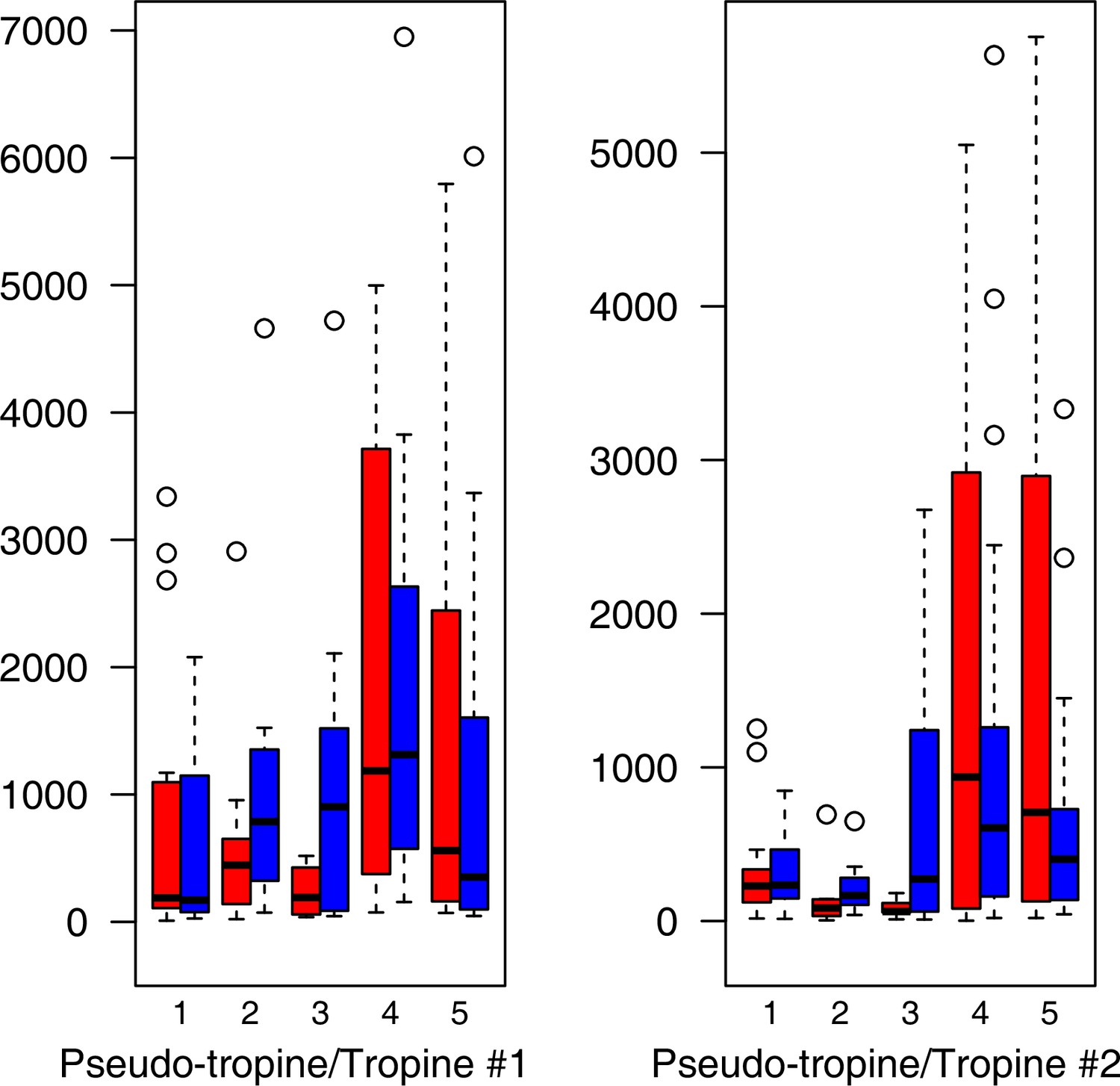
Appendix 1—figure 26
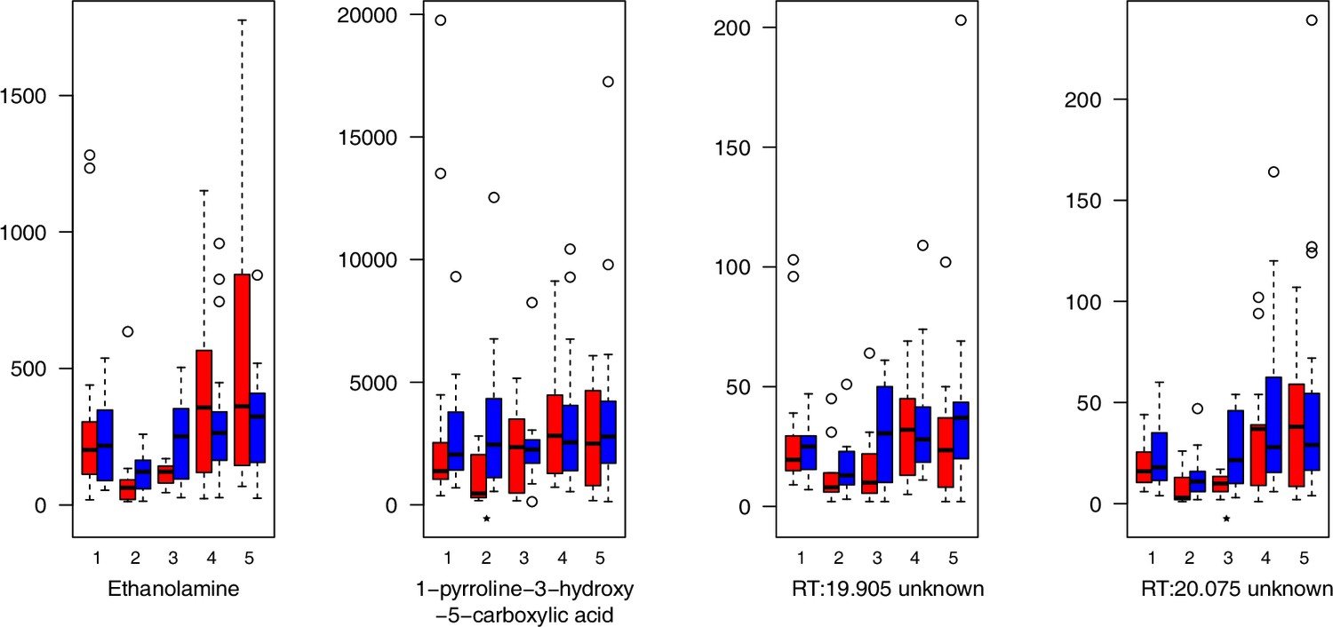
Miscellaneous compounds relative levels (normalized to the ribitol internal standard) under control/cold conditions.
Boxplots showing means of normalized levels to the ribitol internal standard (y-axis) of analyzed miscellaneous compounds in plants from four bioclimatic Cochlearia clusters (x-axis: 1–4; see Figure 4a and b) and Ionopsidium (x-axis: 5) as measured by gas chromatography-mass spectrometry after growing under control (18°C/20°C, red) or cold (5°C, blue) conditions for 20 days. Significant differences between the two treatments within each cluster as revealed via one-way ANOVA are indicated by asterisks (*p≤0.05; **p≤0.02; ***p≤0.001; Appendix 1—figure 22—source data 1). RT, Retention Time in minutes.
Appendix 1—figure 27

Organic acid relative levels (normalized to the ribitol internal standard) under control/cold conditions.
Boxplots showing means of normalized levels to the ribitol internal standard (y-axis) of analyzed organic acids in plants from four bioclimatic Cochlearia clusters (x-axis: 1–4; see Figure 4a and b) and Ionopsidium (x-axis: 5) as measured by gas chromatography-mass spectrometry after growing under control (18°C/20°C, red) or cold (5°C, blue) conditions for 20 days. Significant differences between the two treatments within each cluster as revealed via one-way ANOVA are indicated by asterisks (*p≤0.05; **p≤0.02; ***p≤0.001; Appendix 1—figure 22—source data 1)
Appendix 1—figure 28
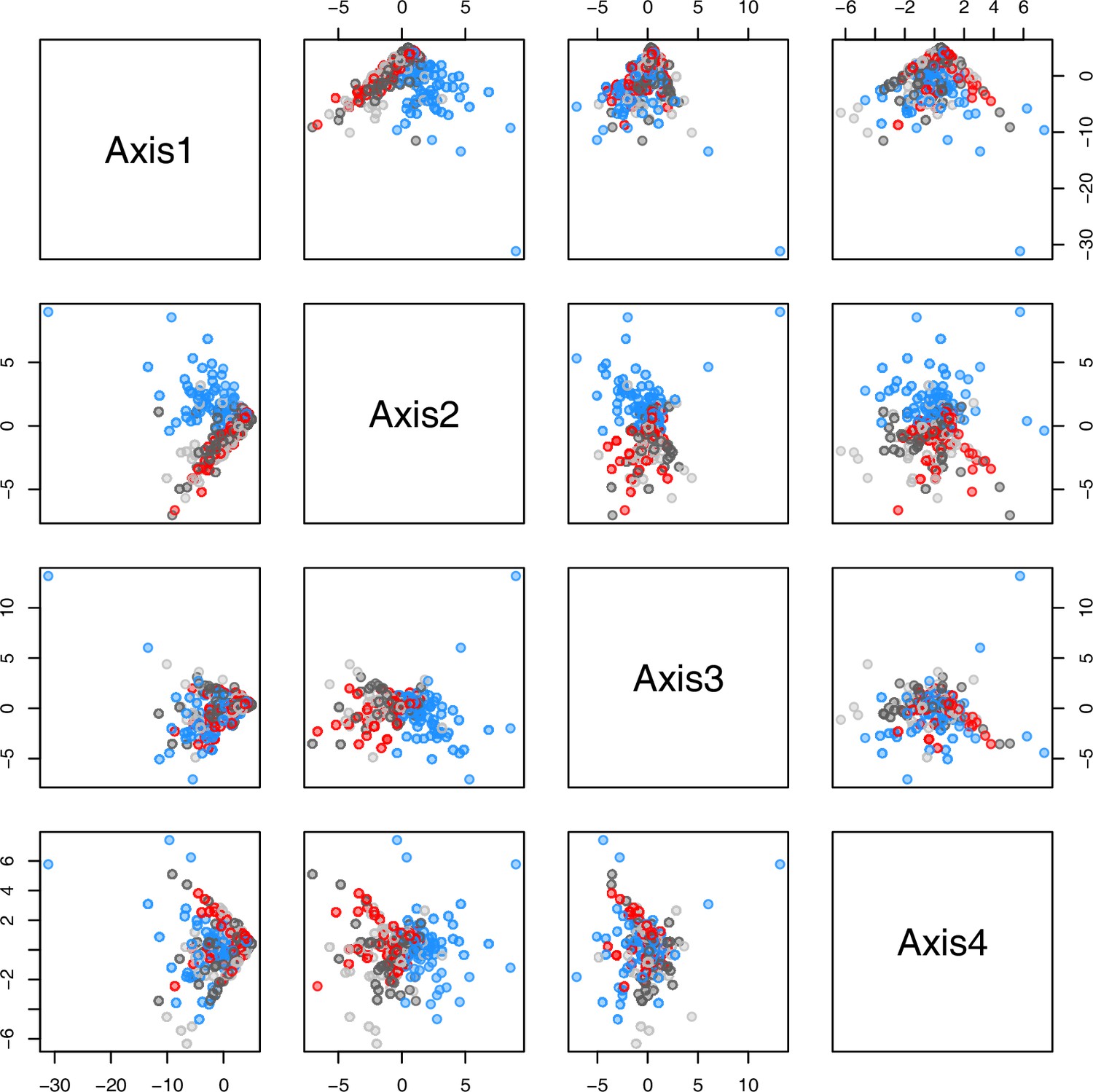
PCA plot of metabolite measurements grouped by treatment.
The first four principal components (Axis1–4) of the normalized metabolite data set grouped by treatment plotted against each other. Colors are representing metabolite extractions as illustrated in Figure 4c. Light/dark grey: plants after the first round of metabolite extractions under control conditions (18°C/20°C) prior to temperature treatment; red: control plants after another 20 days under control conditions; blue: plants after 20 days of cold treatment (5°C).
Appendix 1—figure 29
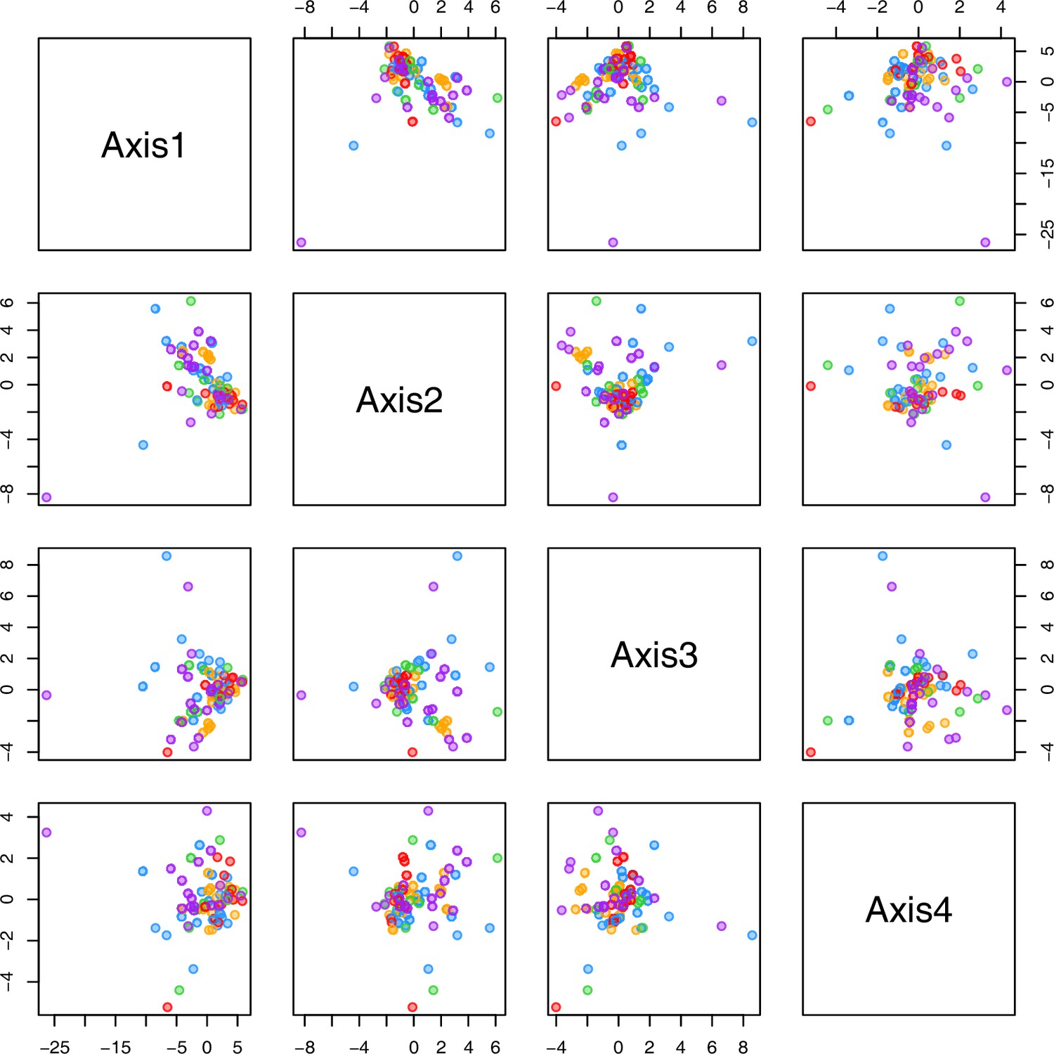
PCA plot of metabolite measurements after cold treatment grouped by bioclimatic clusters.
The first four principal components (Axis1–4) of the normalized metabolite data set grouped by bioclimatic Cochlearia clusters plotted against each other. Colors are representing the four bioclimatic clusters as illustrated in Figure 4a and Ionopsidium (purple).
Appendix 1—figure 30
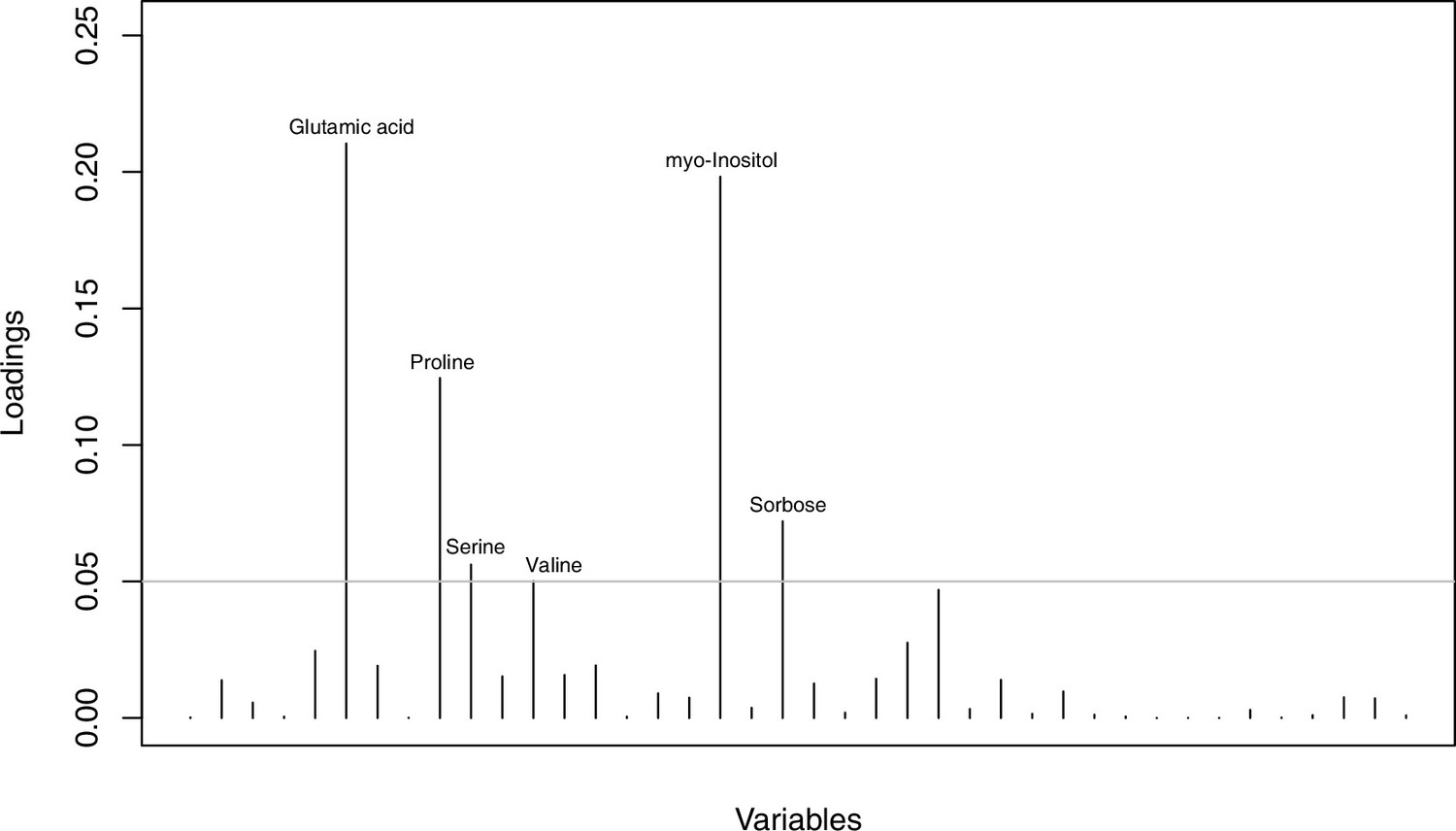
Metabolites with highest discriminating power in DAPC grouped by treatment.
Loading plot of metabolite contributions to discriminant function number 1 (separating control and cold conditions) in DAPC analysis as illustrated in Figure 4d (based on all metabolomic measurements and grouped by treatment). The grey line indicates a threshold of 0.05 and metabolites above this threshold are labeled accordingly. Detailed metabolite contributions given with Appendix 1—figure 30—source data 1.
-
Appendix 1—figure 30—source data 1
Metabolite contributions to discriminant function number 1 (separating control and cold conditions) in DAPC analysis as illustrated in Figure 4d (based on all metabolomic measurements and grouped by treatment) sorted from highest to lowest discriminating power.
- https://cdn.elifesciences.org/articles/71572/elife-71572-app1-fig30-data1-v2.zip
Appendix 1—figure 31
Examples on gating and peak analysis of flow cytometry measurements.
Gating (a) and peak analysis (b) were performed via the Partec FloMax software. Gating was applied as a simple polygon-based gating, defined in the fluorescence channel 1 (FL1) versus side scatter (SSC) dot plot, in order to remove the generally high amount of cellular debris. Samples were stained with propidium iodide (PI) as indicated on the x-axis label. Additional information on corresponding statistics is given with Supplementary Data Set 4.
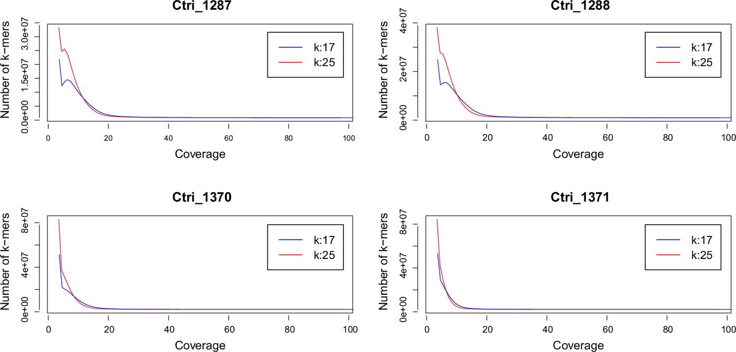
Appendix 2—figure 1
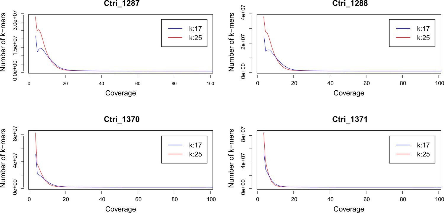
k-mer analysis of sequenced Cochlearia tridactylites samples.
Distribution of k-mers 17 and 25 estimated using Jellyfish (Marçais and Kingsford, 2011).
Additional files
-
Supplementary file 1
Cochlearia species list.
List of accepted Cochlearia taxa according to BrassiBase (Kiefer et al., 2014), in alphabetical order together with information on cytotype, ploidy level, ecology and distribution area.
- https://cdn.elifesciences.org/articles/71572/elife-71572-supp1-v2.xlsx
-
Supplementary file 2
Survey of georeferenced cytogenetic data.
- https://cdn.elifesciences.org/articles/71572/elife-71572-supp2-v2.xlsx
-
Supplementary file 3
Results of chromosome counting and/or flow cytometry measurements.
2C values are given in picograms (pg). Asterisks (*) indicate progeny from open pollination. Chromosome counts marked with ‘FB’ were made on flower buds, generated by Dr. Martin Lysak and Dr. Terezie Mandáková at the Central European Institute of Technology (CEITEC, Brno).
- https://cdn.elifesciences.org/articles/71572/elife-71572-supp3-v2.xlsx
-
Supplementary file 4
Publications considered for cytogenetic literature review.
List of publications (and literature cited therein) screened for Cochlearia chromosome counts and/or genome size measurements.
- https://cdn.elifesciences.org/articles/71572/elife-71572-supp4-v2.xlsx
-
Supplementary file 5
Rank Correlation Analyses.
(1) Correlation between 2C value and chromosome number (full data set, 78 accessions analyzed in total, including putative outliers), (2) Correlation between 2C value and chromosome number excluding Arctic diploids and C. danica as putative outliers (59 individuals, 29 accessions, 11 taxa analyzed in total), (3) Correlation between DNA content per chromosome and total chromosome number (full data set, 78 accessions analyzed in total, including putative outliers), (4) Correlation between DNA content per chromosome and total chromosome number excluding Arctic diploids and C. danica as putative outliers (59 individuals, 29 accessions, 11 taxa analyzed in total).
- https://cdn.elifesciences.org/articles/71572/elife-71572-supp5-v2.xlsx
-
Supplementary file 6
Detailed information on NGS data output and data analyses.
- https://cdn.elifesciences.org/articles/71572/elife-71572-supp6-v2.xlsx
-
Supplementary file 7
Information on accessions selected for Approximate Bayesian Computation (ABC).
For detailed information on selected accessions see Supplementary file 6.
- https://cdn.elifesciences.org/articles/71572/elife-71572-supp7-v2.xlsx
-
Supplementary file 8
Selected population genetic statistics observed for EUR and ARC populations of diploid Cochlearia.
Each statistic is an average over 5601 independent contigs. These statistics together with 103 additional summary statistics formed the basis of the coalescent modeling analyses.
- https://cdn.elifesciences.org/articles/71572/elife-71572-supp8-v2.xlsx
-
Supplementary file 9
Results of model choice via ABC-RF for four models differing in the history of gene flow.
Models explored for the coalescent modeling framework: SI = strict isolation, CM = continuous migration from the population split to the present, OSC = ongoing secondary contact with gene flow starting after population split and continuing up to the present, PSC = past secondary contact with gene flow starting after population split and stopping before the present. The effect of the choice of prior is shown by two different upper bounds of the effective population sizes.
- https://cdn.elifesciences.org/articles/71572/elife-71572-supp9-v2.xlsx
-
Supplementary file 10
Parameter estimates for the SI and OSC models with two choices of priors for the effective population sizes (upper bound of N, Nmax).
The upper part shows medians with 5th and 95th percentiles of the approximated posterior distributions. Population sizes (N) in thousands, time (t) in thousands of generations, and migration rates in log10 of the proportion of immigrants per generation. The lower part shows goodness of fit of these parameter estimates from posterior predictive checks (PPCs), as the standardized euclidean distances between observed summary statistics and predicted values.
- https://cdn.elifesciences.org/articles/71572/elife-71572-supp10-v2.xlsx
-
Supplementary file 11
Accessions included in the metabolomic analyses.
Where possible, missing coordinates were extracted (c.e.) based on information of the respective locality, otherwise coordinates are marked as n/a.
- https://cdn.elifesciences.org/articles/71572/elife-71572-supp11-v2.xlsx
-
Supplementary file 12
SPSS output for KMO and Bartlett’s Test.
- https://cdn.elifesciences.org/articles/71572/elife-71572-supp12-v2.xlsx
-
Supplementary file 13
List of 40 selected metabolic compounds.
Compounds were selected for integration based on annotatability (via the reference collection of the Golm Metabolome Database [GMD, http://gmd.mpimp-golm.mpg.de/] using the AMDIS program [Automated Mass Spectral Deconvolution and Identification System; https://www.amdis.net/]) and reproducibility of peak detection throughout the data set. Metabolites are sorted by general compound classes.
- https://cdn.elifesciences.org/articles/71572/elife-71572-supp13-v2.xlsx
-
Supplementary file 14
Metabolic compound matrix (raw/normalized).
- https://cdn.elifesciences.org/articles/71572/elife-71572-supp14-v2.xlsx
-
Supplementary file 15
Standard plants used for flow cytometric analyses.
Respective 2C-values for Raphanus sativus, Solanum lycopersicum L. cv. ‘Stupické polní rané’ and Glycine max (L.) MERR. cv. ‘
Polanka’ as given in Dolezel et al., 2007.
- https://cdn.elifesciences.org/articles/71572/elife-71572-supp15-v2.xlsx
-
Supplementary file 16
Flow cytometry summary table.
- https://cdn.elifesciences.org/articles/71572/elife-71572-supp16-v2.xlsx
-
Supplementary file 17
Information on mitochondrial DNA sequence reference contigs.
Eight mitochondrial de novo consensus sequences generated from sample Cmica_0979 (Cochlearia micacea) and chosen as reference sequences for mitochondrial genome mappings, with information on contig length and annotated gene content.
- https://cdn.elifesciences.org/articles/71572/elife-71572-supp17-v2.xlsx
-
Supplementary file 18
Prior distributions of the explored ABC models.
SI = strict isolation, CM = continuous migration from the population split to the present, OSC = ongoing secondary contact with gene flow starting after population split and continuing up to the present, PSC = past secondary contact with gene flow starting after population split and stopping before the present. Population sizes (N) in natural units, time (t) in number of generations ago, and migration rates (m) as the fraction of the recipient population made up of immigrants per generation. N parameters were also explored with a higher upper bound, 3 million.
- https://cdn.elifesciences.org/articles/71572/elife-71572-supp18-v2.xlsx
-
Supplementary file 19
SPSS Correlation Matrix of bioclimatic variables.
Correlation table (generated using SPSS version 28) for all 19 standard topo-climatic variables as downloaded for 28 Cochlearia accessions from the high-resolution climate data WorldClim grids at a resolution of 30″ (~1 km²/pixel).
- https://cdn.elifesciences.org/articles/71572/elife-71572-supp19-v2.xlsx
-
Transparent reporting form
- https://cdn.elifesciences.org/articles/71572/elife-71572-transrepform1-v2.docx
-
Appendix 1—figure 2—source data 1
Geographical distribution of ploidy levels in documented Cochlearia accessions.
- https://cdn.elifesciences.org/articles/71572/elife-71572-app1-fig2-data1-v2.zip
-
Appendix 1—figure 4—source data 1
Measured 2C values (in picograms) of all analyzed Cochlearia samples as used for rank correlation analyses (2C value / total chromosome number).
- https://cdn.elifesciences.org/articles/71572/elife-71572-app1-fig4-data1-v2.zip
-
Appendix 1—figure 4—source data 2
Measured 2C values (in picograms) of Cochlearia samples excluding short-lived arctic diploids and the annual C. danica as putative outlier samples as used for rank correlation analyses (2C value / total chromosome number).
- https://cdn.elifesciences.org/articles/71572/elife-71572-app1-fig4-data2-v2.zip
-
Appendix 1—figure 6—source data 1
Best-scoring ML tree based on (nearly) complete plastid genomes and generated in RAxML with 1000 rapid bootstraps.
- https://cdn.elifesciences.org/articles/71572/elife-71572-app1-fig6-data1-v2.zip
-
Appendix 1—figure 7—source data 1
Best-scoring ML tree based on partial mitochondrial genomes and generated in RAxML with 1000 rapid bootstraps.
- https://cdn.elifesciences.org/articles/71572/elife-71572-app1-fig7-data1-v2.zip
-
Appendix 1—figure 8—source data 1
Tanglegram nexus-file (plastome versus mitochondrial sequence data).
- https://cdn.elifesciences.org/articles/71572/elife-71572-app1-fig8-data1-v2.zip
-
Appendix 1—figure 12—source data 1
Best-scoring ML tree based on transcriptome-wide nuclear SNPs (298,978 variant sites) and generated in RAxML with an ascertainment bias correction and 1000 rapid bootstraps.
- https://cdn.elifesciences.org/articles/71572/elife-71572-app1-fig12-data1-v2.zip
-
Appendix 1—figure 13—source data 1
STRUCTURE result C. bavarica at K=2 (uncorrelated allele frequency model).
- https://cdn.elifesciences.org/articles/71572/elife-71572-app1-fig13-data1-v2.zip
-
Appendix 1—figure 13—source data 2
STRUCTURE result C. bavarica at K=2 (correlated allele frequency model).
- https://cdn.elifesciences.org/articles/71572/elife-71572-app1-fig13-data2-v2.zip
-
Appendix 1—figure 19—source data 1
Bootstrapped (100 bootstrap replicates) maximum likelihood consensus tree generated with TreeMix with one migration/admixture event.
- https://cdn.elifesciences.org/articles/71572/elife-71572-app1-fig19-data1-v2.zip
-
Appendix 1—figure 20—source data 1
19 WorldClim bioclimatic variables for 28 Cochlearia accessions.
- https://cdn.elifesciences.org/articles/71572/elife-71572-app1-fig20-data1-v2.zip
-
Appendix 1—figure 21—source data 1
11 WorldClim bioclimatic variables for 28 Cochlearia accessions.
- https://cdn.elifesciences.org/articles/71572/elife-71572-app1-fig21-data1-v2.zip
-
Appendix 1—figure 22—source data 1
Detailed summary output of one-way ANOVAs for all metabolites for bioclimatic clusters (1–4) and Ionopsidium (5).
- https://cdn.elifesciences.org/articles/71572/elife-71572-app1-fig22-data1-v2.zip
-
Appendix 1—figure 30—source data 1
Metabolite contributions to discriminant function number 1 (separating control and cold conditions) in DAPC analysis as illustrated in Figure 4d (based on all metabolomic measurements and grouped by treatment) sorted from highest to lowest discriminating power.
- https://cdn.elifesciences.org/articles/71572/elife-71572-app1-fig30-data1-v2.zip
Download links
A two-part list of links to download the article, or parts of the article, in various formats.
Downloads (link to download the article as PDF)
Open citations (links to open the citations from this article in various online reference manager services)
Cite this article (links to download the citations from this article in formats compatible with various reference manager tools)
Evolutionary footprints of a cold relic in a rapidly warming world
eLife 10:e71572.
https://doi.org/10.7554/eLife.71572


