Juxtacellular opto-tagging of hippocampal CA1 neurons in freely moving mice
- Institute of Neurobiology, Eberhard Karls University of Tübingen, Germany
- Werner-Reichardt Centre for Integrative Neuroscience, Germany
- Graduate Training Centre of Neuroscience – International Max-Planck Research School (IMPRS), Germany
- Chinese Academy of Sciences, Key Laboratory of Brain Connectome and Manipulation, The Brain Cognition and Brain Disease Institute, Shenzhen Institute of Advanced Technology, Chinese Academy of Sciences, China
- Shenzhen-Hong Kong Institute of Brain Science-Shenzhen Fundamental Research Institutions, China
Figures
Figure 1 with 1 supplement
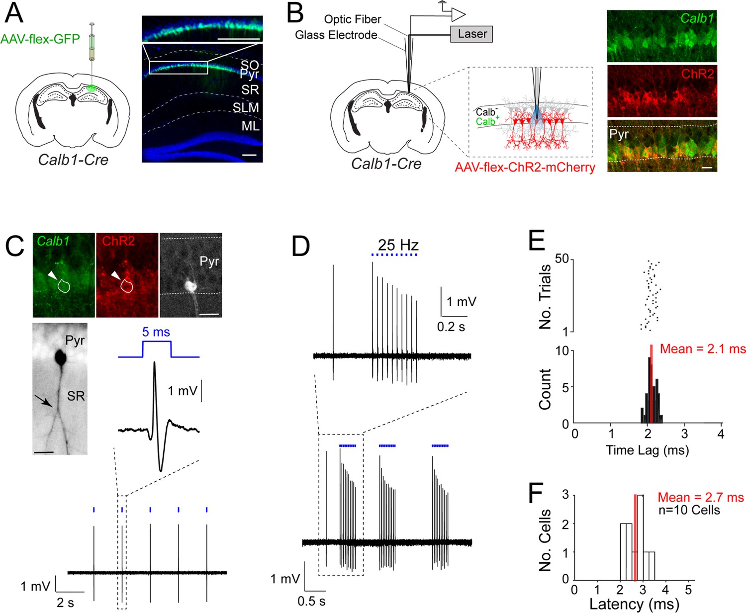
Juxtacellular opto-tagging of Calb1-positive CA1 pyramidal cells in anesthetized mice.
(A) Left, a schematic of a mouse coronal brain section showing the injection site of AAV-CAG-flex-GFP in Calb1cre mice. Right, epifluoresence image showing Green Fluorescent Protein (GFP) expression (green) in the superficial pyramidal cell layer (blue, DAPI). SO, stratum oriens; Pyr, stratum pyramidale; SR, stratum radiatum; SLM, stratum lacunosum moleculare; ML, molecular layer of dentate gyrus. Scale bar = 100 µm. (B) Left, a schematic of a mouse coronal brain section showing the juxtacellular opto-tagging recording configuration. Right, a confocal image showing the expression of mCherry coexpressed with ChR2 (red) in the superficial Calb1-positive pyramidal layer (green). Scale bar = 20 µm. (C) A representative light-responsive pyramidal neuron, recorded in vivo. Top, epifluorescence images showing Calb1 (green), ChR2 (red), and Neurobiotin labeling of the neuron (white). Middle, z-stack projection of the same neuron (inverted signal). The arrowhead indicates a branching point of the primary apical dendrite. Bottom, high-pass filtered juxtacellular spike trace, showing short-latency spike responses upon pulses of blue light (5 ms, indicated in blue). Scale bar = 20 µm. (D) Bottom, high-pass filtered juxtacellular spike traces of a representative neuron responding to 25 Hz light-pulse stimuli. Top, high-magnification view on a single train (25 Hz, 10 pulses). (E) Raster plot (top) and peristimulus time histogram (bottom) showing the spike latency to the light stimulus for the neuron shown in C. The average latency is indicated. (F) Histogram of average spike latencies of all identified Calb1-positive pyramidal neurons in CA1 (n = 10).
-
Figure 1—source data 1
Juxtacellular opto-tagging data, average spike latencies (source data for panels E and F).
- https://cdn.elifesciences.org/articles/71720/elife-71720-fig1-data1-v1.xlsx
Figure 1—figure supplement 1
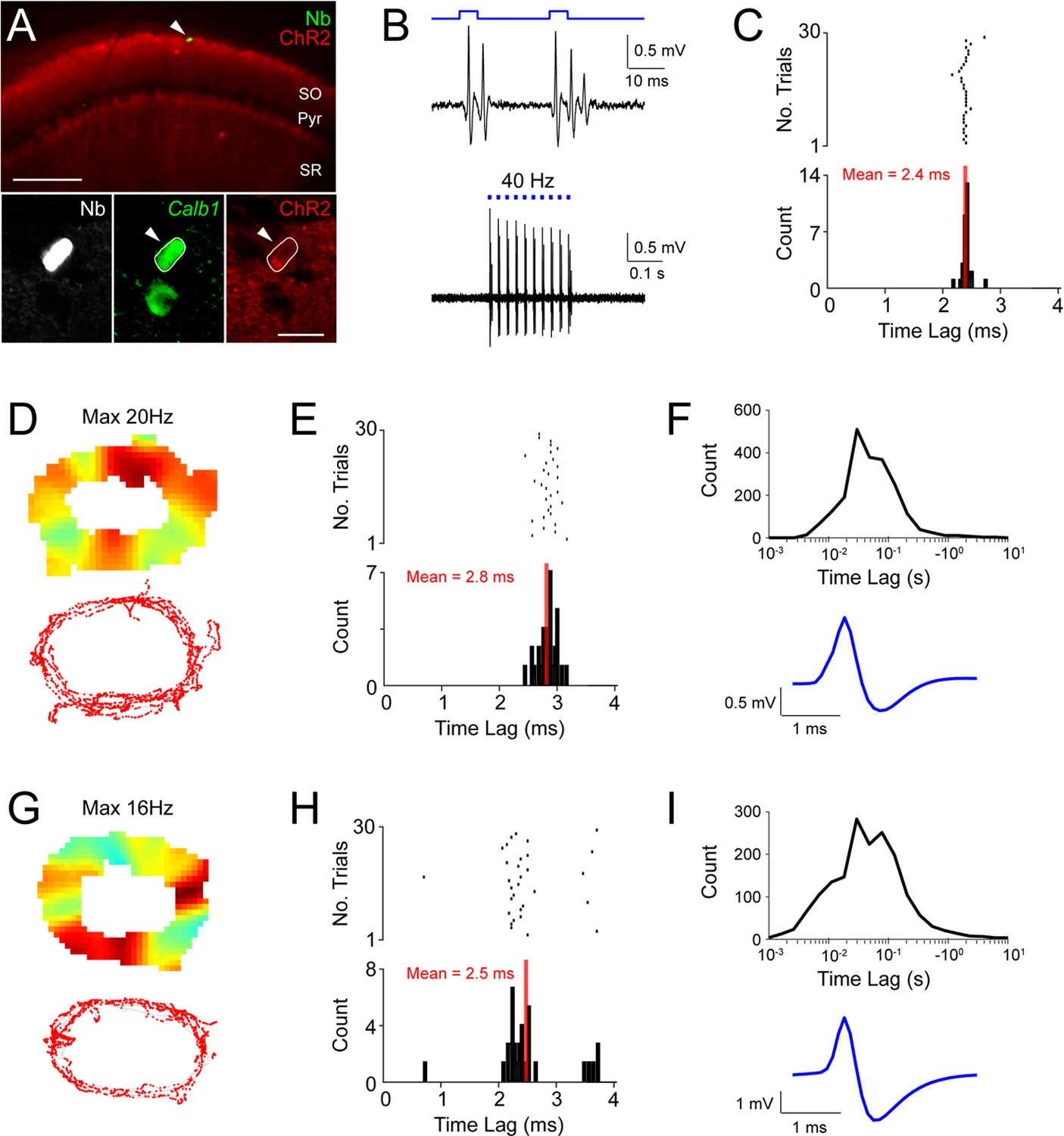
Juxtacellular opto-tagging of Calb1-positive interneurons in the CA1 region.
(A) Epifluorescence images showing a Calb1-positive interneuron recorded, opto-tagged and identified in an anesthetized mouse (Neurobiotin, white; Calb1, green; ChR2, red). Scale bar = 200 µm (top) and 20 µm (bottom). (B) Bottom, high-pass filtered juxtacellular spike traces of the neuron shown in (A) responding to 40 Hz trains of light pulses. Top, high-magnification view on two light pulses. (C) Raster plot (top) and peristimulus time histogram (bottom) showing the spike latency to the light stimulus for the neuron shown in (A). The average latency is indicated. (D) Color-coded rate map (top) and spike-trajectory plot (bottom) of a putative Calb1-positive interneuron recorded in a freely moving mouse. (E) Same as (C) but for the interneuron shown in (D). (F) The distribution of interspike intervals (top) and average spike waveform for the putative Calb1-positive interneuron shown in (C). (G–I) Same as (D–F), but for another putative Calb1-positive interneuron.
-
Figure 1—figure supplement 1—source data 1
Electrophysiological properties of putative Calb1-positive interneurons (source data for panels C,E,F,H,I).
- https://cdn.elifesciences.org/articles/71720/elife-71720-fig1-figsupp1-data1-v1.xlsx
Figure 2
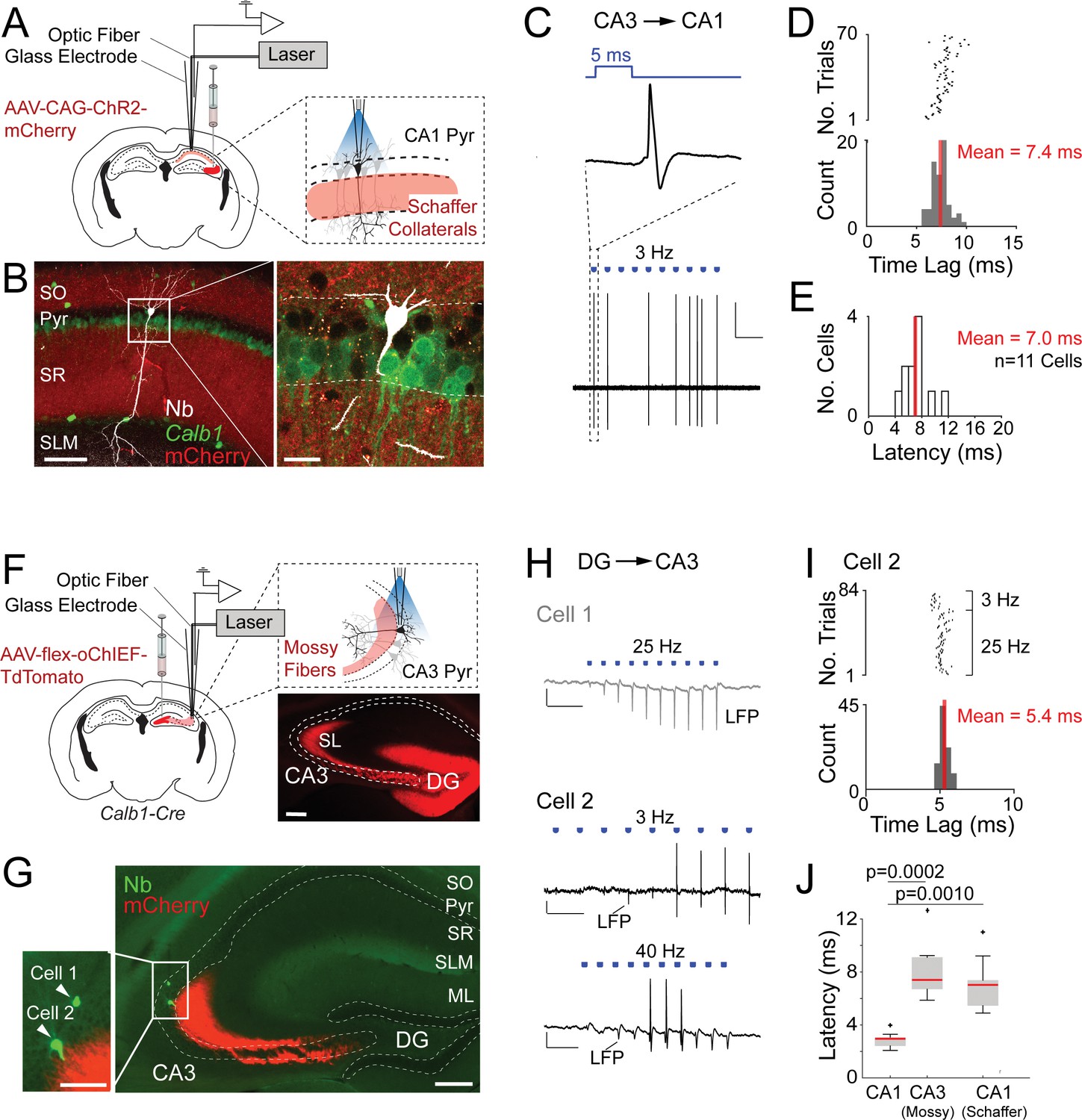
Juxtacellular opto-activation of Schaffer collaterals and mossy fiber inputs onto postsynaptic neurons in anesthetized mice.
(A) Left, schematic of a mouse coronal brain section showing the injection site of an opsin-expressing viral vector (AAV-CAG-ChR2-mCherry) in the CA3 region. Right, schematic showing the opto-activation of Schaffer collateral inputs combined with juxtacellular recording from single CA1 pyramidal neurons. (B) Confocal images showing a light-responsive CA1 pyramidal neuron (recording shown in C, D) labeled in vivo. Right panel, high-magnification view on the neuron (white, Neurobiotin, Nb) relative to the labeled Schaffer collaterals (red, ChR2-mCherry) and Calb1 staining (green). Scale bars = 100 µm (left), 20 µm (right). (C) High-pass filtered juxtacellular trace (bottom) for the neuron shown in B. Note the partial spiking responses to the light pulses (3 Hz, ~1.3 mW). Top, high magnification showing long-latency spike responses upon pulses of blue light (5 ms, indicated in blue). Scale bar = 2 mV, 2 s. (D) Raster plot (top) and peristimulus time histogram (bottom) showing the spike latency to the light stimuli for the CA1 pyramidal neuron shown in B. The average latency is indicated. (E) Histogram of average spike latencies of CA1 neurons (n = 11) showing spiking responses to Schaffer collateral input activation. The average latency is indicated. (F) Left, schematic of a mouse coronal brain section showing the injection site of recombinase-dependent opsin-expressing viral vectors (e.g., AAV-EF1a-flex-ChR2-eYFP, AAV-hSyn1-flex-ChR2-mCherry, or AAV-hSyn1-flex-oChIEF-TdTomato) in the dentate gyrus of Calb1cre mice. Right top, schematic showing the opto-activation of mossy fiber inputs combined with juxtacellular recording from single CA3 pyramidal neurons. Right bottom, epifluorescence image showing eYFP signal (pseudocolored to red for display purposes) following the injection of AAV-CAG-flex-eYFP. Note the labeling of mossy fibers (red) along the transverse CA3 axis. DG, dentate gyrus; SL, stratum lucidum; SO, stratum oriens; Pyr, stratum pyramidale; SR, stratum radiatum; SLM, stratum lacunosum moleculare; ML, molecular layer of dentate gyrus. Scale bar = 200 µm. (G) Epifluorescence image showing a nonresponsive (Cell 1) and a responsive (Cell 2) CA3a pyramidal neuron, recorded (as in F) along the same electrode penetration and labeled in vivo. Left panel, high magnification on the somata of the two neurons (green, Nb) relative to the labeled mossy terminals (red, oChIEF-TdTomato). Scale bars = 100 µm (left inset), 200 µm (right). (H) Representative recordings from the nonresponsive (Cell 1) and responsive (Cell 2) CA3a pyramidal neurons shown in G. The recording form Cell 1 (top, gray) shows the absence of spiking, but increasing amplitude of the negative local field potential (LPF) deflection during the stimulus train (25 Hz, 5-ms pulse duration) − consistent with the expected facilitation of neurotransmitter release at mossy terminals. Scale bars = 2 mV, 100 ms. The recording from Cell 2 (middle and bottom, black) shows partial spiking responses to low and high-frequency light pulses (3 and 40 Hz, 5 ms). Note the increase of the local field potential (LFP) amplitude (indicated with an arrow) during the stimulus trains. Scale bars = 2 mV, 500 ms (middle trace); 2 mV, 50 ms (bottom trace). (I) Raster plot (top) and peristimulus time histogram (bottom) showing the spike latency to the light stimuli for Cell 2 shown in G,H. 40 Hz light stimulus trains were excluded because of a high probability of spiking failure (see details in Materials and Methods). The average latency is indicated. (J) Boxplots showing comparison of latencies between directly activated CA1 cells (n = 10), indirectly activated CA3 (via mossy fiber photostimulation, n = 7), and CA1 cells (via Schaffer collateral photostimulation, n = 11). Significant p values after multiple group comparison are indicated (Kruskal–Wallis, p = 0.00006). Red lines indicate medians. Outliers are shown as crosses.
-
Figure 2—source data 1
Juxtacellular opto-tagging data, average spike latencies (source data for panels D,E and I,J).
- https://cdn.elifesciences.org/articles/71720/elife-71720-fig2-data1-v1.xlsx
Figure 3 with 2 supplements

Juxtacellular opto-tagging of single CA1 pyramidal neurons in freely moving mice.
(A) Schematic drawing of the fully assembled recording implant for juxtacellular opto-tagging in freely moving mice (adapted from Diamantaki et al., 2018). (B) Raster plots (top) and peristimulus time histograms (bottom) showing responses from a Calb1-positive (left) and Calb1-negative (right) neuron to the light stimulus (indicated in blue). Note the short-latency spiking of the Calb1-positive neurons (mean latency indicated) and the absence of response in the Calb1-negative cell. (C) Reconstruction of the dendritic morphology of a Calb1-negative CA1 pyramidal neuron, recorded in a freely moving mouse (recording shown in E). Scale bar = 50 µm. (D) Epifluorescence image showing Calb1 staining (green) and the juxtacellular labeled CA1 neuron (Neurobiotin, red) for the neurons shown in C. Scale bar = 20 µm. (E) Rate map (top) and spike-trajectory plot (bottom) for the neuron shown in (C). (F–H) Same as in (C–E) but for a representative Calb1-positive CA1 pyramidal neuron. (I) Linearized rate maps of all Calb1-negative cells (n = 26) that met the inclusion criteria for spatial analysis (see Materials and Methods). Each row represents the normalized firing rates relative to the linearized 1D projection of the circular arena. Cells are ordered according to their maximal firing rate position along the linearized trajectory. The bar graph on the right indicates peak firing rates (‘Peak FR’) for each cell, calculated from the original, non-linearized rate maps. (J) Same as in (I) except for all Calb1-positive cells (n = 12) that met the inclusion criteria for spatial analysis (see Materials and Methods). (K) Boxplots showing spatial information content and sparsity for Calb1-negative (n = 26, as in I) and Calb1-positive (n = 12, as in J) CA1 neurons. p values are indicated (Wilcoxon rank-sum test). Black/green lines indicate medians. Outliers are shown as crosses.
-
Figure 3—source data 1
Electrophysiological properties of Calb1-positive and Calb1-negative neurons (source data for panels I-K and Figure 3—figure supplement 2K).
- https://cdn.elifesciences.org/articles/71720/elife-71720-fig3-data1-v1.xlsx
Figure 3—figure supplement 1
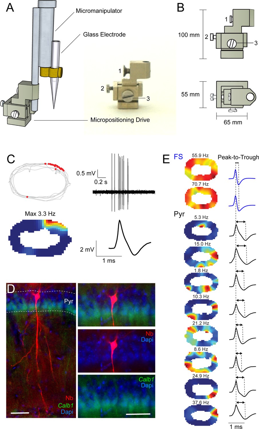
Mechanical micropositioning drive enables multiple juxtacellular recordings within individual animals.
A known limitation of previous juxtacellular procedures in freely moving animals (Tang et al., 2014a; Diamantaki et al., 2018) is that – following implantation of the recording components – the position of the recording electrode relative to the craniotomy cannot be easily adjusted by the experimenter. De facto, this limits the number of electrode penetrations (and recording/labeling attempts) that can be performed within an individual craniotomy, since consecutive electrode penetrations cannot be efficiently and systematically spaced relative to each other. To circumvent this limitation, we have developed a mechanical micropositioning system that enables adjusting the electrode’s position prior to recording. A representative experiment showing multiple recordings from CA1 neurons obtained during sequential electrode penetrations in the same craniotomy is shown in (C–E). (A) Left, 3D schematic representations of the microdrive/micromanipulator assembly for obtaining juxtacellular recordings in freely moving mice. The base of the micropositioning drive (image shown on the right panel) is cemented on the mouse’s head (not shown). By means of a positioning Screw (2), the mechanical microdrive allows the displacement of the electrode along the horizontal plane (100 μm per turn), thereby allowing spacing (and differentiating) multiple electrode penetrations along one dimension (maximum travel distance, 1 mm). (B) Side and top views of the micropositioning drive (dimensions are shown). Screw (1) secures the microdrive to the motorized micromanipulator (Diamantaki et al., 2018); Screw (2) is the positioning screw (see A); Screw (3) secures the microdrive components after the Screw (2) has been operated. (C) A representative recording from an identified CA1 place cell, recorded in a freely moving mouse. Left, color-coded rate map (top) and spike-trajectory plot (bottom) showing spatially localized activity. Peak firing rate is indicated. Right, high-pass filtered juxtacellular spike traces (top) and averaged spike waveform (bottom). (D) Epifluoresence image showing the CA1 pyramidal neuron (Nb, red) recorded in a freely moving mouse (recording shown in C). The neuron was located in the deep CA1 layer, and was negative for Calb1 expression (green). Red, Neurobiotin (Nb); green, Calb1; blue, DAPI. Scale bar = 50 µm. (E) Color-coded rate maps (left; peak firing rates indicated) and average spike waveforms (right) for the recordings performed in the same animal as the cell in (C, D). These recordings included two putative fast-spiking (FS) interneurons and eight additional putative pyramidal (Pyr) neurons. Note the higher firing rates and shorter spike peak-to-trough times for the FS, compared to Pyr recordings.
-
Figure 3—figure supplement 1—source data 1
Average spike waveforms (source data for panels C and E).
- https://cdn.elifesciences.org/articles/71720/elife-71720-fig3-figsupp1-data1-v1.xlsx
Figure 3—figure supplement 2
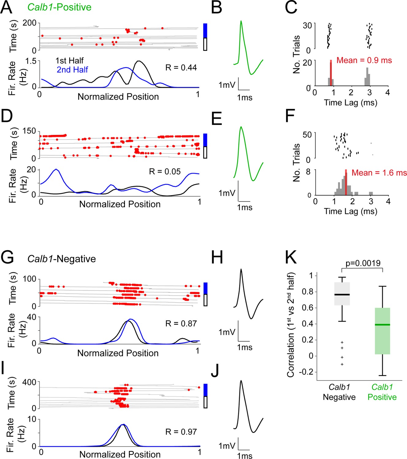
Stability analysis of spatial firing in Calb1-postive and Calb1-negative neurons.
(A) Representative recording from a putative Calb1-positive neuron, recorded in a freely moving mouse (recording configuration as in Figure 3A). Linearized spike-trajectory (top) and firing rates (bottom) computed for the first half (black) and second half (blue) of the recording. Pearson’s correlation coefficient (R) is indicated. (B) Average spike waveform for the recording shown in (A). (C) Raster plot (top) and peristimulus time histogram (bottom) showing the spike latency to the light stimuli for the recording shown in (A). The average latency is indicated. (D–F) Same as (A–C), but for another putative Calb1-positive neuron. (G–J) Same as in (A–E), but for two putative Calb1-negative neurons. (K) Boxplot showing Pearson’s correlation coefficients between the rate maps computed for the two halves of each Calb1-positive (n = 12) and Calb1-negative (n = 26) recording. p values are indicated (Wilcoxon rank-sum test). Black/green lines indicate medians. Outliers are shown as crosses.
Author response image 1
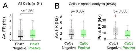
Average and peak firing rates of Calb1-positive and Calb1-negative neurons.
(A)Box plots showing average firing rates for all Calb1-positive (n=15) and Calb1-negative neurons (n=39) recorded in freely moving animals (B) Average and Peak firing rates for the subset of neurons included in the spatial analysis (n=12 Calb1positive, n=26 Calb1-negative neurons; see Materials and methods).
Additional files
Download links
A two-part list of links to download the article, or parts of the article, in various formats.
Downloads (link to download the article as PDF)
Open citations (links to open the citations from this article in various online reference manager services)
Cite this article (links to download the citations from this article in formats compatible with various reference manager tools)
Juxtacellular opto-tagging of hippocampal CA1 neurons in freely moving mice
eLife 11:e71720.
https://doi.org/10.7554/eLife.71720


