A parameter-free statistical test for neuronal responsiveness
- Netherlands Institute for Neuroscience, Royal Netherlands Academy of Arts and Sciences, Netherlands
Figures
Figure 1
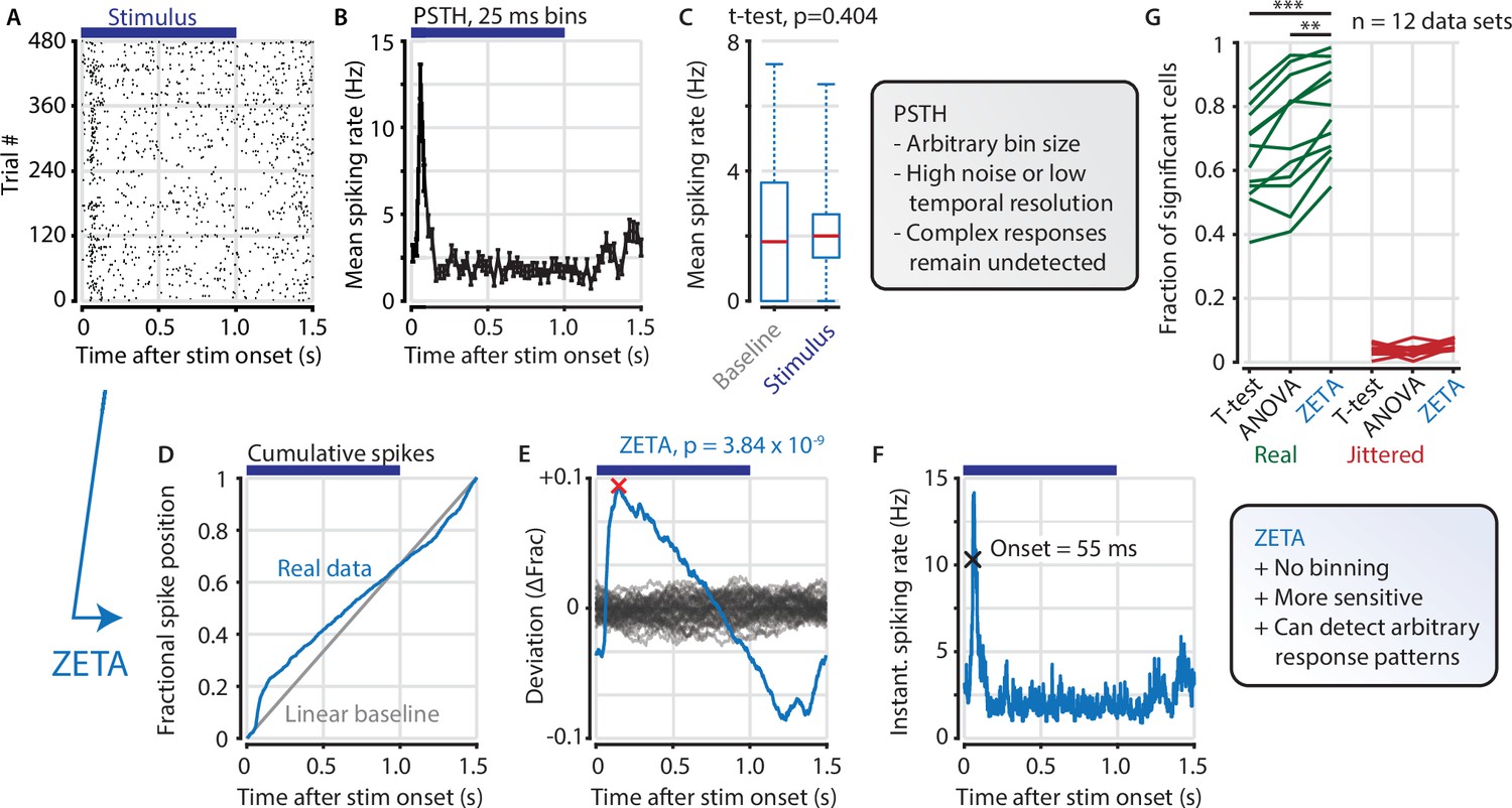
The ZETA-test detects an example visually responsive neuron in V1.
(A,B) Raster plot (A) and PSTH (B) for a neuron that shows an onset peak and a reduced sustained spiking in response to a visual stimulus (purple bars). (C) A common approach for computing a neuron’s responsiveness is to perform a t-test on the average activity per trial during stimulus presence (0–1 s) and absence (1.0–1.5 s), which fails to detect this neuron’s response (paired t-test, p = 0.404, n = 480 trials). (D) ZETA avoids binning, by using the spike times to construct a fractional position for each spike (blue) and compares this with a null-distribution of a stationary rate (grey). (E) The difference between the real and null curves gives a deviation from expectation (blue), where the most extreme value is defined as the Zenith of Event-based Time-locked Anomalies (ZETA, red cross). To compute its statistical significance (here, p = 3.84 × 10⁻⁹), we compare ZETA to the variability over repeats of the procedure with jittered onsets (grey curves). (F) A ZETA-derived instantaneous spiking rate allows a reliable estimation of response onset. (G) At a significance threshold of α = 0.05, ZETA detects more stimulus-responsive cells than both a mean-rate t-test (***: paired t-test, p = 2.8 x 10⁻⁷, n = 12 data sets) and an ANOVA over bins using an optimal bin width (**: p = 0.0014).
Figure 2 with 1 supplement
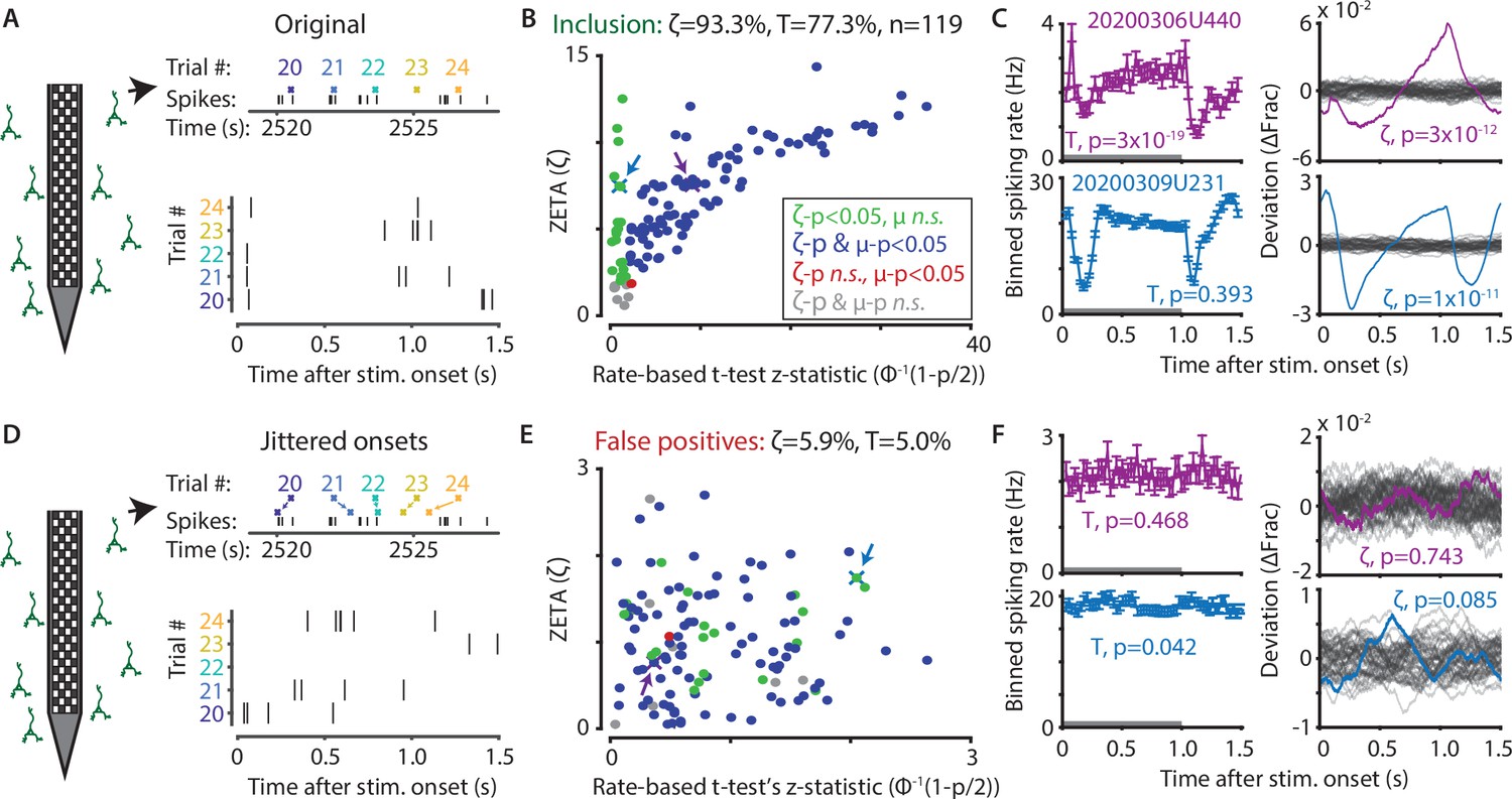
The ZETA-test outperforms the t-test for V1 neurons (n = 119).
(A) Spikes were recorded with neuropixels in mouse V1 and aligned with the onset of square-wave drifting gratings. (B) Applying the ZETA-test, we found that 93.3 % of all V1 neurons showed significant firing rate modulations that were time-locked to stimulus onset. Using a rate-based t-test between stimulation (0–1 s) and no stimulation (1–1.5 s) epochs across trials registered 77.3 % of neurons to be visually responsive. Neurons detected by only ZETA are green, by both methods are blue, by only a mean-rate t-test are red, and by neither are grey. Arrows indicate the neurons shown in C. (C) Two example neurons that are (1) detected by a rate-based t-test as well as ZETA (top) and (2) not detected by a rate-based t-test, but only by ZETA (bottom). (D) We investigated the false-positive rate of both approaches by jittering the onsets of visual stimuli; this preserved the temporal structure of the spiking response, but destroys the time-locked modulations in activity. (E–F) same cells and analyses as in B-C but for jittered onsets. Red indicates neurons included by ZETA, but not a t-test; green indicates neurons included by a t-test, but not ZETA. As expected, the percentage of false positives (i.e., neurons with ζc/z-statistic > 2.0) was around 5 % (α = 0.05) for both approaches. Note the change in axis magnitude from B to E.
Figure 2—figure supplement 1
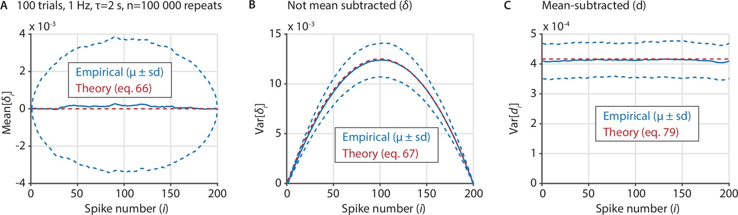
Several important variables underlying the ZETA-test can be derived analytically in the case of exponentially-distributed inter-spike intervals.
(A) We sampled 100,000 artificial neurons with exponentially-distributed inter-spike intervals, each spiking at 1 Hz during 100 trials that last 2 s. To compile data over neurons, we interpolated the spike position to [1 200], regardless of the real number of spikes. Blue shows the mean ± standard deviation of the mean of δi for each spike number i, while the theoretical prediction is shown in red. (B) Same as A, but for the variance of δi as a function of i. (C) Same as B, but after recentering δ to mean-zero, showing the variance of di as a function of i.
Figure 3 with 4 supplements
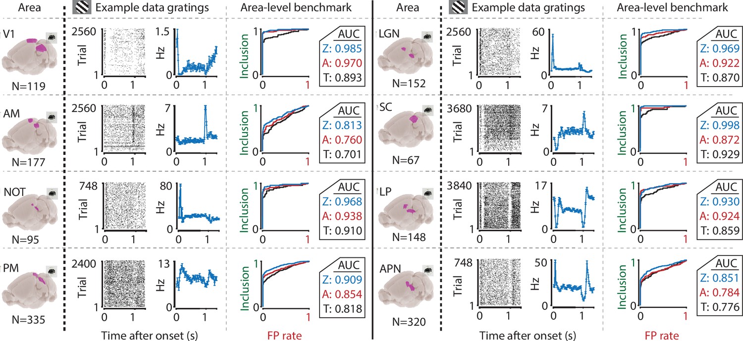
The ZETA-test’s superior sensitivity is independent of brain area.
We recorded neuronal responses to drifting gratings (1 s with 500 ms blank ITIs) from various visual brain areas: V1, SC, AM, LP, NOT, APN, PM, and LGN. For each area, we show an example neuron’s raster plot (left) and binned responses (right). All cells depicted here were significant using ZETA. Area-level benchmark summaries show ROC analyses of the inclusion rate (y-axis) and false-positive (FP) rate (x-axis) for ZETA (Z, blue), bin-wise ANOVA (A, red), and rate-based t-tests (T, black). In all cases, the AUC of the ZETA-test exceeded both the ANOVA’s AUC and t-test’s AUC.
Figure 3—figure supplement 1
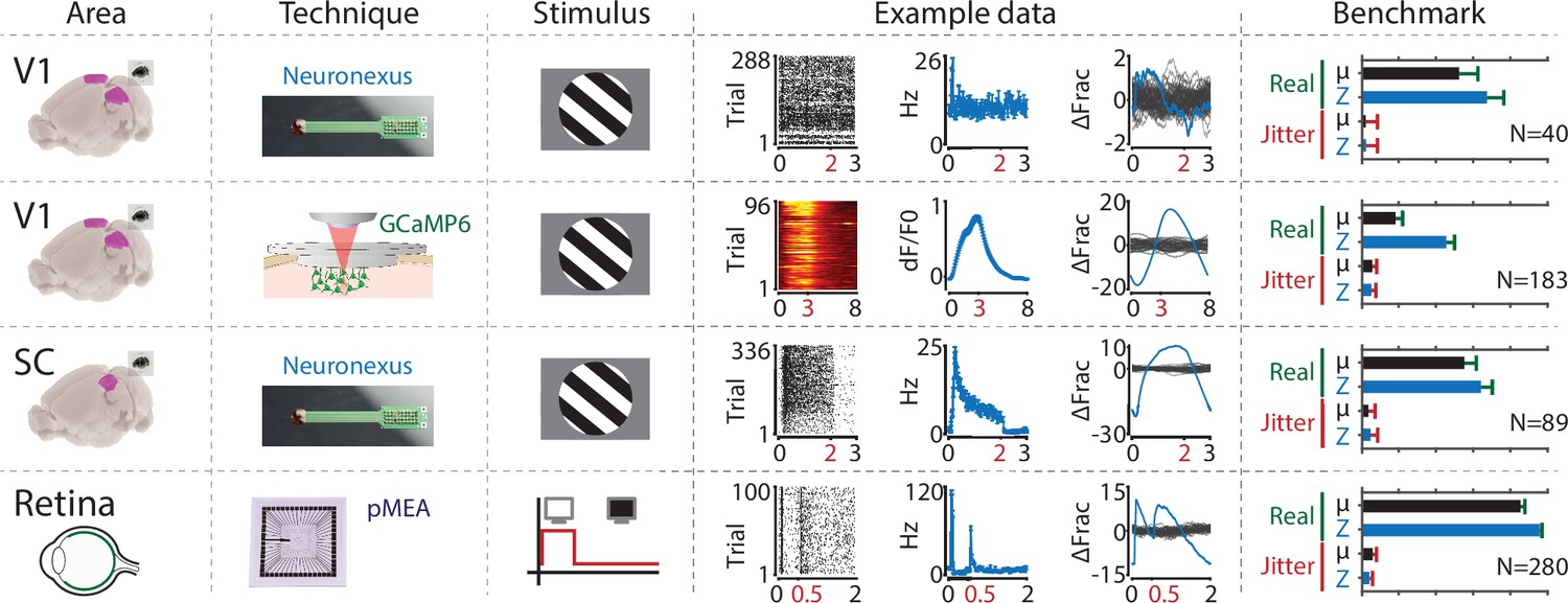
The ZETA-test is more sensitive than a mean-rate approach across a range of areas, recording techniques and stimuli.
From left to right the figure shows the following. First column: the recorded area. Second column: recording technique. Third column: stimulus. Fourth column: example data including raster plot or heat map (lhs), neural activity in spiking rate (Hz) or dF/F0 (middle) and activation deviation (rhs, ΔFrac). All cells depicted here were significant using ZETA. Fifth column: benchmark performance for neuronal inclusion percentage (‘Real’, green) and false alarm rate after jittering (‘Jitter’, red) for tests using mean-rate (black, µ) and ZETA (blue, Z). From top to bottom, we investigated several data sets: mouse V1 responses to drifting gratings recorded with a Neuronexus probe (top row) and GCaMP6f (second row), mouse superior colliculus responses to drifting gratings recorded with a Neuronexus probe (third row), and zebrafish retinal ganglion cell responses to on/off light flashes recorded with a perforated micro-electrode array (fourth row). Bar graphs show inclusion rate and 75th percentile confidence interval.
Figure 3—figure supplement 2
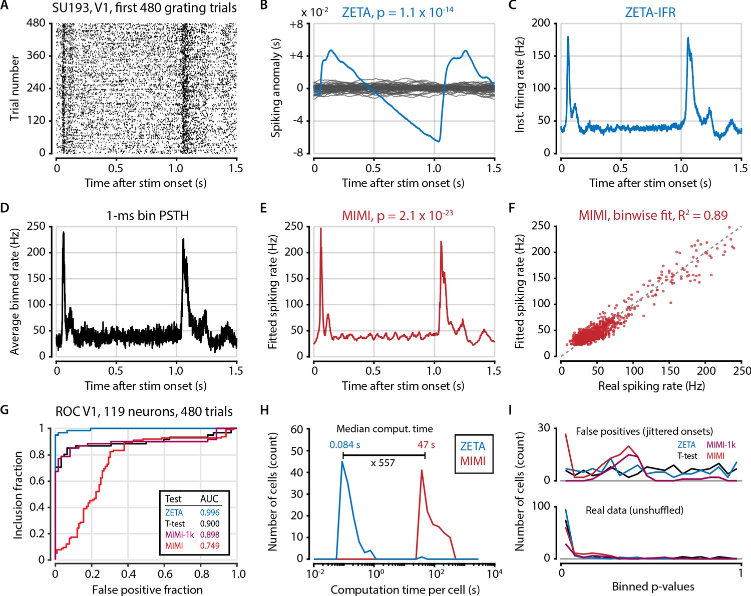
Model-based methods require high spike counts or hyperparameter tuning.
(A) Raster plot of example (high firing rate) V1 cell. Because of the prohibitively long computation time of fitting a multiplicative inhomogeneous Markov interval (MIMI) model to the data we opted to use only the first 480 trials recorded for each cell (N = 119 neurons in V1 from two animals). (B) Spiking anomaly (blue) and shuffle controls (grey) for the same cell, showing a clear stimulus-locked response. (C) The instantaneous firing rate captures the neuron’s spiking response very well. (D) 1 ms binning provides a similar time resolution to both the IFR-method (panel C) and the MIMI-fit (panel E) but is much noisier at the level of single bins. (E) The MIMI-model fit also captures the neuron’s spiking response well (see F). Statistical significance with the MIMI-model fit was determined by calculating bin-wise d’ values from the confidence intervals at each 1 ms bin (see Materials and methods). (F) The MIMI-model fit explains a large proportion of the variance of the PSTH (R2 = 0.89 for this example cell), but still underperforms when used as the basis for a statistical test for stimulus-responsiveness (see panel G). (G) ROC analysis showing the performance of the ZETA-test, t-test, and two versions of the MIMI-model fit. While the MIMI-model fitting worked well for cells with high spiking rates, cells with low firing rates were prone to spurious low p values during shuffle controls (see panel I). While the base MIMI-model gave an AUC of 0.749 (versus 0.996 of ZETA), excluding cells with fewer than 1,000 spikes during this 480-trial epoch increased the MIMI-model’s performance to on-par with the t-test (t-test AUC = 0.900, MIMI-1k AUC = 0.898). The threshold of 1000 spikes corresponds to an average firing rate of 1.38 Hz. (H) In addition to performing worse than the ZETA-test, the MIMI-method was also much more computationally intensive: the median computation time was 557 times longer than for the ZETA-test. (I) Distribution of p-values for real data (top) and shuffled controls (bottom) for the four tests; note that excluding cells with low firing rates removes all of the MIMI’s false positives.
Figure 3—figure supplement 3
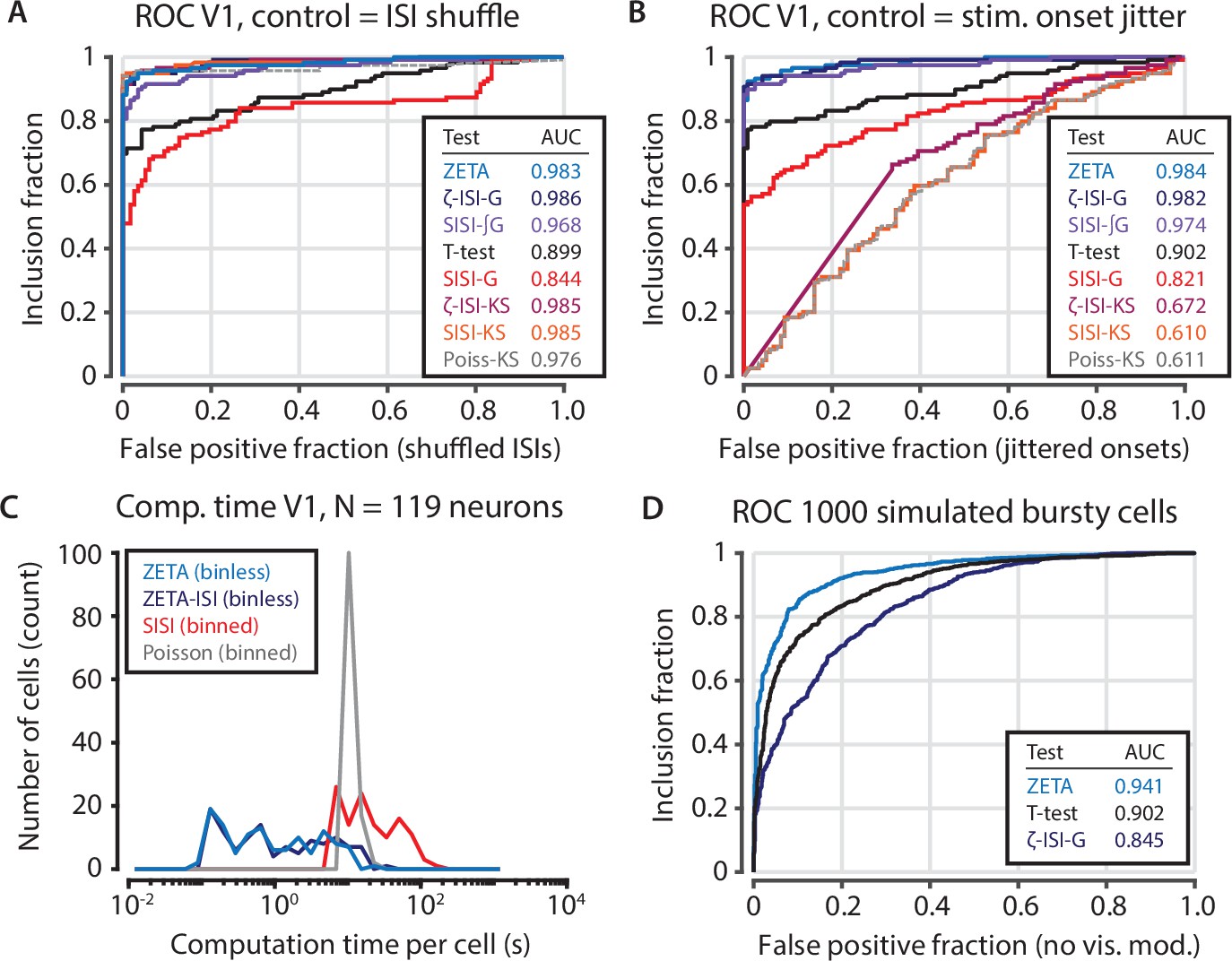
Intermediate statistical tests reveal the functions of the components of the ZETA-test.
(A) Various forms of statistical tests; most perform well when the test’s null distribution matches the real distribution of the unresponsive population (shuffled inter-spike intervals). (B) When the test’s assumed (shuffled ISIs) and real (jittered onsets) null distributions are different, the Kolmogorov-Smirnov based tests fail. Of the remaining tests, the ZETA-test and ISI-shuffle ZETA-test perform best. Note that the difference in performance with Figure 3—figure supplement 2 is due to different data selection. (C) Bin-based tests (SISI, Poisson) are slower than binless tests (ZETA, ZETA-ISI). (D) Although the ZETA-test and ISI-shuffle ZETA-test performed similarly for data sets with mostly regular spiking cells (panels A,B), the ISI-shuffle ZETA-test performs considerably worse in differentiating stimulus-modulated from unmodulated bursty cells; ZETA-test AUC = 0.941; Mean-rate t-test AUC = 0.902; ISI-shuffle ZETA-test AUC = 0.845.
Figure 3—figure supplement 4
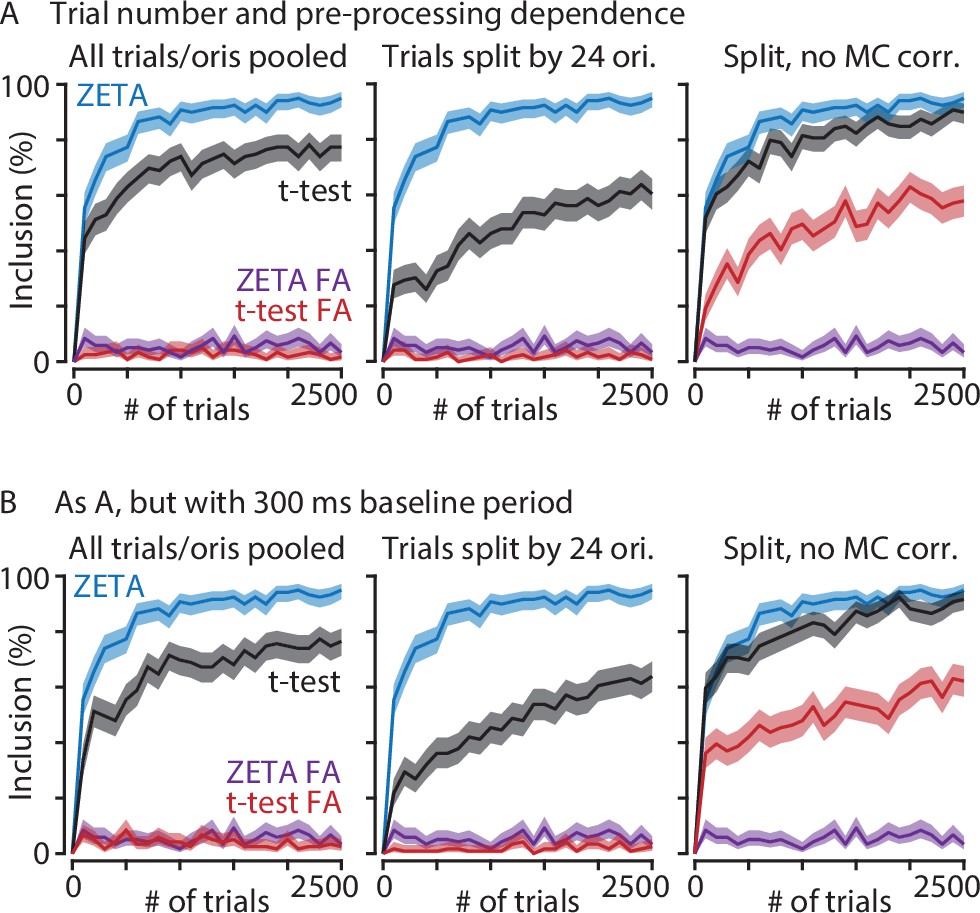
The ZETA-test performs better than t-tests at low trial numbers and regardless of data preparation.
(A) Graphs show V1 inclusion percentage as a function of number of trials subsampled from the whole data set, using the ZETA-test (blue) and t-test (black), and false alarms after jittering using the ZETA-test (purple) and t-test (red). Left-hand panel shows results when trials of all orientations are pooled. Middle and right-hand panels show results when t-test p-values are calculated separately per orientation (24 groups) and Bonferroni-corrected (middle) or not corrected (right). (B) As panel A, but now using a 300 ms window preceding stimulus onset as baseline. There is little difference in t-test performance between using a 300 ms or 500 ms window. In all cases, the ZETA-test performs better than t-tests.
Figure 4

The t-test exceeds the ZETA-test’s performance only in the hypothetical case of purely Poisson-distributed spike counts and only for a small range of spiking rate differences.
(A) Top: the ability of the t-test to differentiate simulated stimulus (non)modulated cells depends only the total spike count during stimulus (0–1 s) and inter-trial interval (ITI, 1–2 s) periods (x axis; firing rate difference d(Hz)), but not on the duration of the cell’s response when keeping the spike count constant (y axis; response duration T). Bottom: in contrast, the ZETA-test can differentiate stimulus modulation using either variable. (B) Top: example PSTHs of single cells corresponding to the markers 1–4 in (A). Bottom: ROC curves for the combination of variables marked as 1–4 in (A). The ZETA-test always exceeds the t-test’s performance, except for a limited range where the response duration is 1 s. (C) A more biologically plausible test case is bursting neurons that have an elevated probability of bursting during stimuli. (D–E) This simulation produces no ‘onset’ peaks of activity that the ZETA-test can exploit. (F) However, despite the lack of clear peaks of activity, the ZETA-test exceeds the t-test’s ability to detect stimulus-modulated bursting cells (ZETA AUC = 0.941, t-test AUC = 0.902).
Figure 5
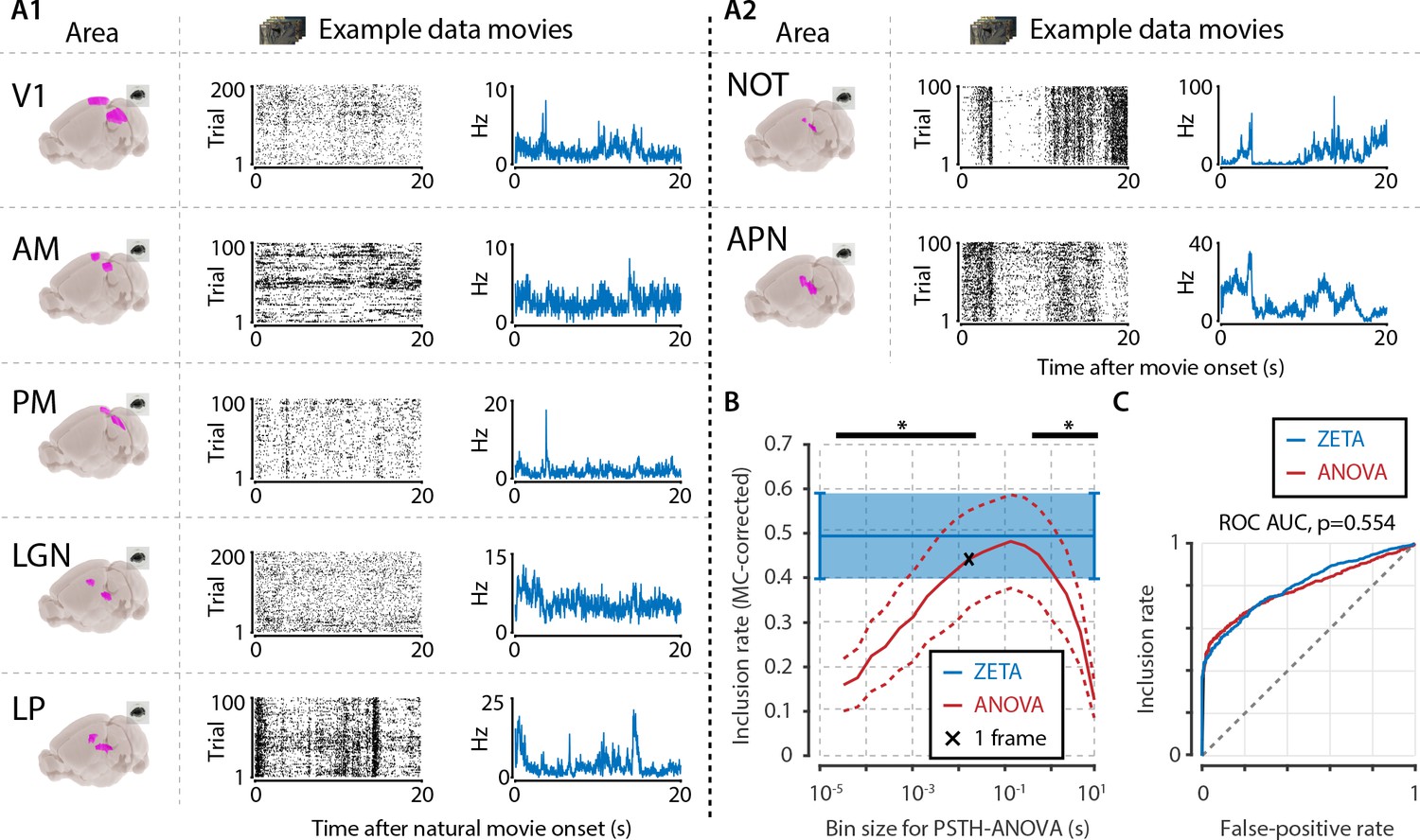
Determining neuronal responsiveness to natural movies.
(A) We recorded neuronal responses to natural movies (four scenes that repeated every 20 s) from various visual brain areas: V1, AM, PM, LGN, LP, NOT, and APN. For each area, we show an example neuron’s raster plot (left) and binned responses (right). All cells depicted here were significant using ZETA. (B) We determined a neuron’s responsiveness using a 1-way ANOVA over all binned responses (i.e. PSTH-level ANOVA) for various bin sizes and MC-corrected (black) and using the ZETA-test (blue). Note that the ZETA-test is timescale-free and plotted at all x-values only for easy comparison with the ANOVAs. Curves show mean ± SEM over brain regions (n = 7). ZETA shows an inclusion rate similar to the most optimal bin sizes (0.0333s – 0.2667s), and significantly higher than bin sizes of 0.0167 s or shorter, as well as 0.533 s or longer (*, FDR-corrected paired t-tests, p < 0.05). (C) An ROC analysis on all n = 977 cells showed that the ZETA-test and a combined set of ANOVAs were similarly sensitive (ZETA-test AUC: 0.792 ± 0.011; ANOVAs AUC: 0.798 ± 0.010; z-test, p = 0.554).
Figure 6
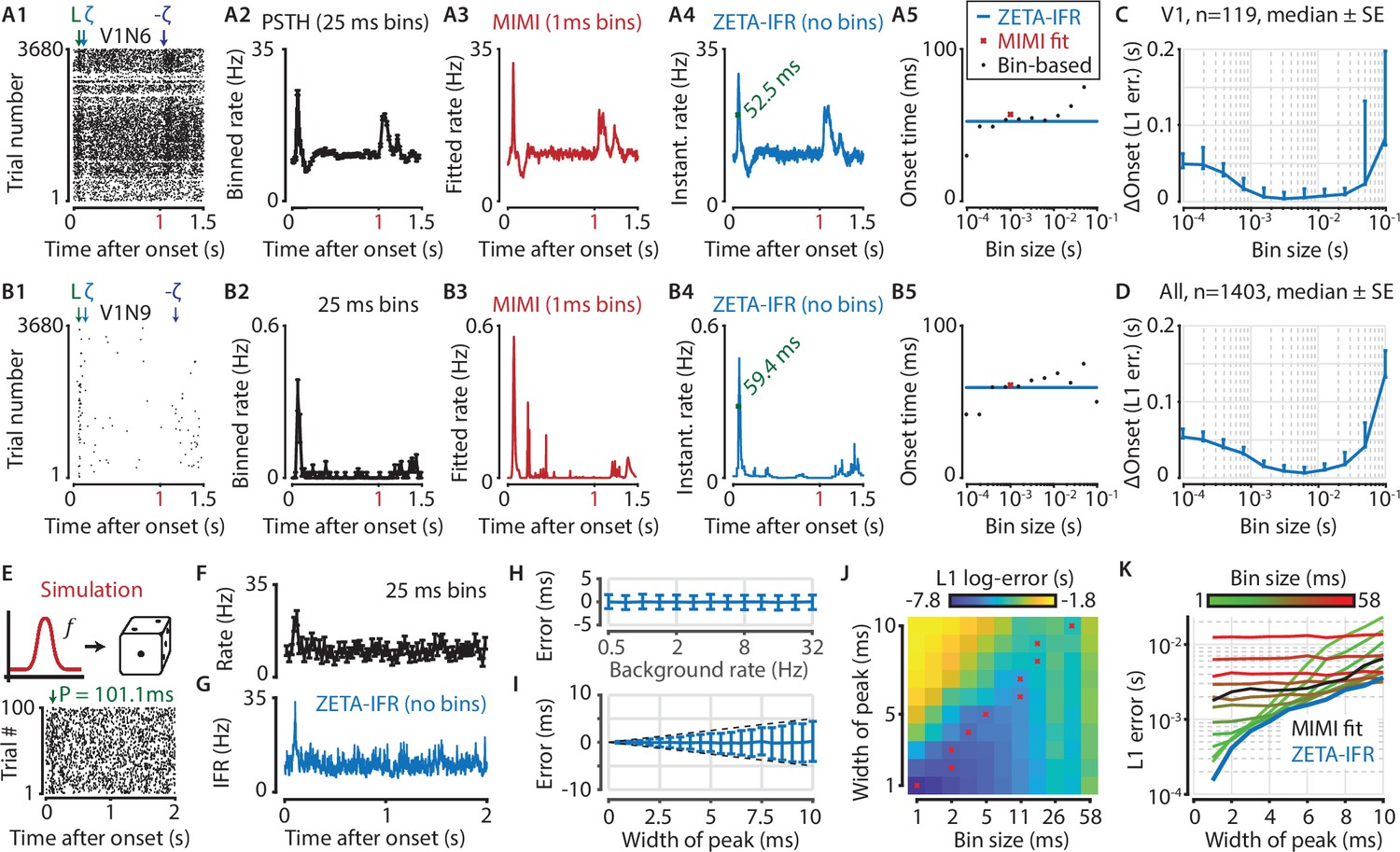
A ZETA-derived measure for instantaneous firing rates (IFR) avoids binning and allows more accurate latency determination than with PSTHs.
(A,B) Responses of two example V1 cells to drifting gratings. From left to right: (1) Raster plots showing the estimated onset latency (‘L’, green), and times of ZETA (blue) and –ZETA (purple). (2) Spiking rates using 25 ms bins. (3) Spiking rates using multiplicative inhomogeneous Markov interval (MIMI) model-based fits. (4) Binning-free instantaneous spiking rates provide a much higher temporal resolution. Using the first crossing of half-peak firing rates, we determined the onset latencies of these cells to be 52.5 and 59.4 ms. (5) Estimated onset times using our method for instantaneous firing rates (blue), MIMI model-based fits (red), or PSTHs with bin widths from 0.1 to 100 ms (black). Onset latency estimates depend on the chosen bin size, and the optimal size varies across cells. (C–D) The median (± SE) difference in onsets estimated by our instantaneous firing rates compared to that of various sized bins for V1 cells (C, n = 119) and for cells from all brain regions (D, n = 1403). Both C and D show the onsets estimated by the two methods were most similar for bin sizes between 1–10 ms. (E–K) Benchmarking of peak detection using artificial Poisson neurons that show a transient peak. (E) Example Poisson cell for a background rate of 10 Hz and a peak-width of 10 ms. With the true peak at 100 ms, the estimation error here was 1.1 ms. (F) Binning the cell’s spiking response in 25 ms bins reduces the peak height and temporal precision. (G) Our instantaneous spiking rate preserves a sharper peak response and allows for a temporally accurate latency estimation. (H) The detection of peak latencies is insensitive to realistic levels of a stationary Poisson background firing rate (13 base rates, 0.5–32 Hz). (I) The mean error is unbiased, and the standard deviation in the onset peak latency estimate scales linearly with the width of the peak. Dotted lines show the real peak width. Graphs in H-I show mean ± sd. (J) The error in peak latency estimation depends on both the bin width and the width of the neuron’s peak response. Red crosses indicate the bin size with the lowest error for a given peak width. (K) Plotting the latency estimation error shows that different bin sizes (red-green) are optimal for different peak-widths. The accuracy of the latency obtained from MIMI-based fits (black) is less sensitive to the peak width, but never performs as well as well as the most optimal bin size. The error based on our binning-less IFR (blue) is as at least as low as the most optimal bin size, for any peak width.
Figure 7 with 1 supplement
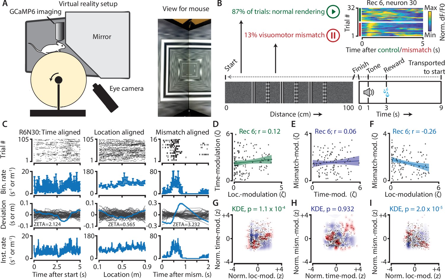
Neurons in V1 encode either visuomotor mismatch signals or spatial location.
(A) Schematic of setup showing mouse on running wheel (lhs) viewing a virtual tunnel (rhs). (B) Trials consist of a 100 cm linear track. One second after the mice ran to the end of the tunnel, an auditory stimulus signaled that a water reward would be delivered two seconds later. 6 s after reward delivery, mice were transported to the start of the virtual tunnel. In a subset of trials, the rendering of the tunnel was paused at a random location, eliciting a visuomotor mismatch signal. Top right shows calcium imaging data for an example ‘mismatch neuron’ during 16 control and 16 mismatch trials. (C) Spiking data for example neuron obtained from exponential fits of the dF/F0 signals. Putative spikes were aligned to start (left), location of the animal on the track (middle), or mismatch onset (right). From top to bottom: raster plot of putative spike times; mean ± SEM of firing rates over trials (n = 105 trials, of which n = 16 mismatch trials); spiking deviation underlying ZETA; instantaneous firing rate. (D–I) Relationship between time-, location-, and mismatch-modulation. One point is one neuron. (D–F) ZETA-scores for example recording 6 (N = 120 neurons). (G–I) Analysis using a kernel-density estimate (KDE) to test whether joint-encoding of two features is more common than expected by chance (see Figure 1). (G) More neurons showed joint-encoding of both spatial and temporal location than expected by chance (p = 1.1 × 10⁻⁴). (H) Joint-encoding of temporal location and mismatch was not significantly different from chance (p = 0.932). (I) Location on the virtual track and visuomotor mismatch are less likely to be encoded by the same neuron than expected from chance (p = 2.0 × 10⁻⁵). See Figure 7—figure supplement 1 for more details on the KDE procedure.
Figure 7—figure supplement 1
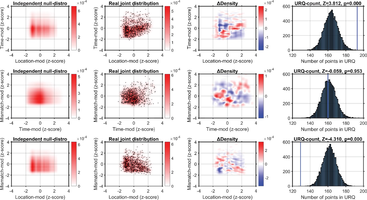
Using a kernel-density estimator (KDE) to investigate the joint-encoding of two features.
Each column shows one step in our analysis procedure, and each row shows the comparison of two features. Top row shows the comparison of location-modulation (x-axis) with time-modulation (y-axis). Left-hand panel: probability density derived from combining the independent KDE-distributions of location-modulation and time-modulation. Middle-left panel: real joint probability distribution (red-scale). One point is a single neuron’s modulation after z-scoring per recording. Middle-right panel: the difference in probability density between the real and null-hypothesis distributions. Blue indicates fewer neurons in the real joint-distribution than in the null-hypothesis distribution. The upper-right quadrant is mostly red, indicating the real distribution contains more neurons that encode both location and time than expected by chance. Right-hand panel: we sampled 10,000 synthetic neuronal populations from the null-hypothesis probability distribution, and calculated for each synthetic population the number of neurons that fell in the upper-right quadrant (URQ): that is, the number of neurons that show both above-average location-modulation as well as above-average time-modulation. The histogram shows the number of neurons in the URQ for each of the 10,000 populations, and the blue vertical line shows that the real number of neurons in the URQ is much higher than expected by chance (z = 3.812, p = 1.144 × 10⁻⁴). Middle row: as top row, but now comparing time- and mismatch-modulation. The URQ-analysis showed that time- and mismatch-modulation were not more often seen in the same neurons than expected by chance if the two features are independently encoded (z = −0.059, p = 0.953 (n.s.)). Bottom row: location on the virtual track and visuomotor mismatch are less likely to be encoded by the same neuron than if the two features were randomly distributed (z = −4.310, p = 2.019 × 10⁻⁵). This shows that neurons show an encoding specialization for either spatial location or visuomotor mismatch, but not both. Analyzing the Pearson correlation per recording we find qualitatively similar results. Mean Pearson correlation between time-modulation and location-modulation across recordings: n = 7, mean r = 0.2272; one-sample t-test vs. 0: p = 0.0164. Mean correlation between time- and mismatch-modulation: r = 0.1267, p = 0.2829 (n.s.). Mean correlation between location- and mismatch-modulation: r = −0.2249, p = 0.0414.
Figure 8
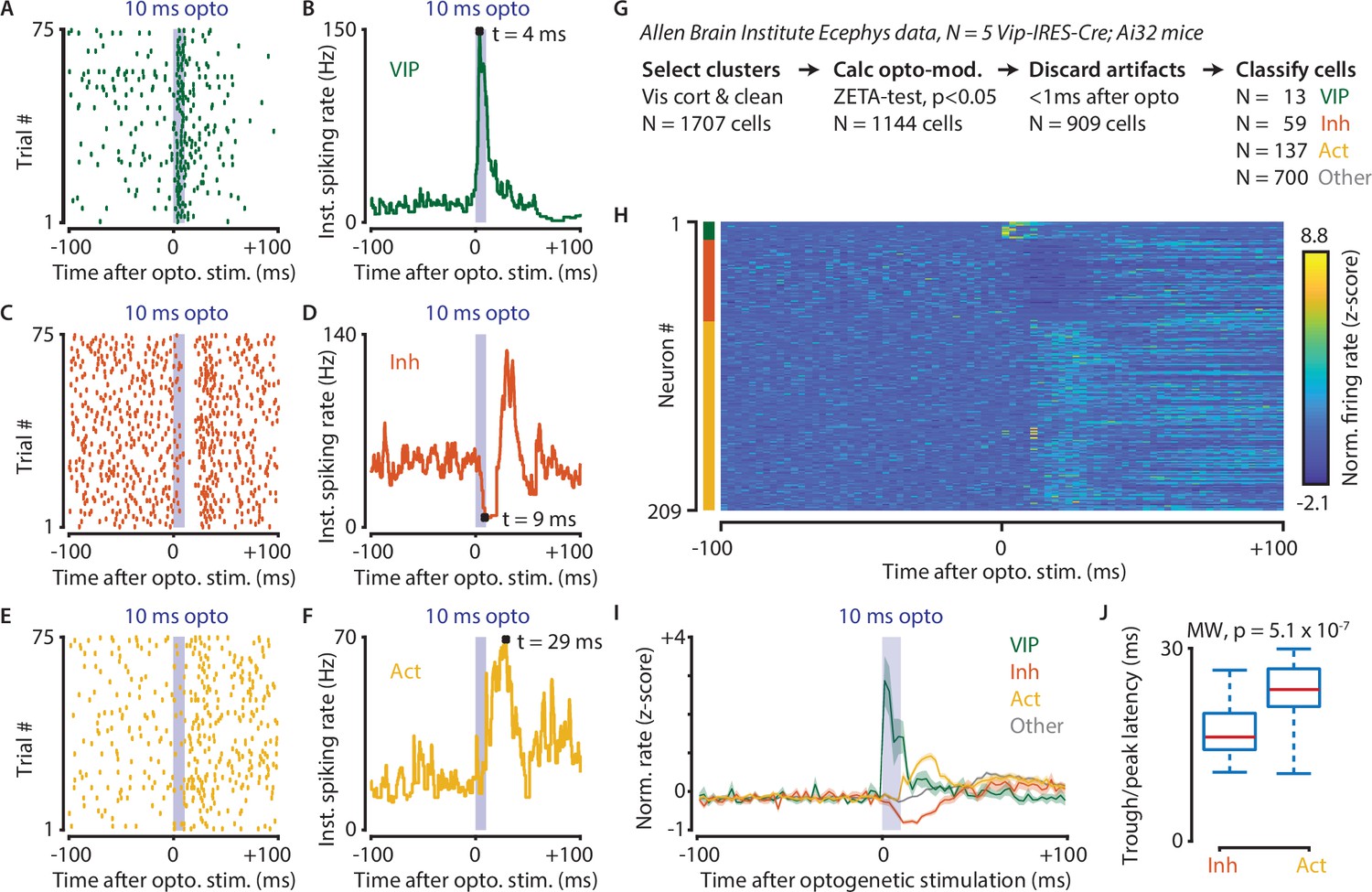
Optogenetic stimulation of VIP-expressing cells in mouse visual cortex causes short-latency inhibition and longer latency disinhibition of the local neural circuit.
(A–F) Response of example cells classified as VIP (A,B), Inhibited (C,D) and Activated (E,F). (G) Data were recorded in visual cortex from 5 Vip-Cre mice at the Allen Brain Institute. Cells were only included if the clustering quality was sufficient (1707 cells total). A ZETA-test included cells that were modulated within (–0.5, + 0.5 s) after optogenetic stimulation (N = 1144 cells). IFR peak- and trough-latency was computed and cells were discarded if their peak was earlier than 1 ms after optogenetic stimulation onset. Remaining cells were classified as VIP (N = 13), Inhibited (N = 59), Activated (N = 137), or Other (N = 700). (H) Heat map showing normalized firing rate of VIP (top), Inhibited (middle), and Activated (bottom) cells. (I) Mean ± SEM of PSTH (2.5 ms bin size) over all VIP (green), Inhibited (orange), Activated (yellow), and Other (gray) cells. (J) Inhibited cells showed significantly lower mean IFR-peak latencies after optogenetic stimulation than Activated cells (Inh: 17.4 ms; Act: 23.0 ms; Mann-Whitney U-test, p = 5.1 × 10⁻⁷).
Tables
Table 1
Parameters of bursting neurons used in Figure 4.
Abbreviations and mathematical symbols are as follows: ISI = Inter-spike interval; IBI = Inter-burst interval; Exp = exponential distribution; |x| = absolute of x; N = standard normal distribution; U(x,y) = uniform distribution on interval [x,y]; ℳ = von Mises distribution; Γ = Gamma distribution.
| Property | Unit | Distributed as | Sampled from: |
|---|---|---|---|
| Single-spike ISI | s | Exp(1 /r) | r~Exp(λ = 1) |
| Baseline IBI | s | Exp(1/| Rb|) | Rb~|N|/20 + 1/80 |
| Preferred orientation IBI | s | Exp(1/| Rt|) | Rt~|N| + 1/4 |
| Preferred orientation | rad | θp | θp~U(0,2π) |
| Orientation-tuned bursting | Hz | 1/Rb + 1/Rt ∙ ℳ(θp, κ) | κ ~ 5 + U(0,5) |
| Burst duration | ms | Γ(2*k, θ = 0.5) | k~90 + 10*N |
| ISI in bursts | ms | Γ(2*k, θ = 0.5) | k~0.5 + Exp(λ = 2.4) |
Additional files
Download links
A two-part list of links to download the article, or parts of the article, in various formats.
Downloads (link to download the article as PDF)
Open citations (links to open the citations from this article in various online reference manager services)
Cite this article (links to download the citations from this article in formats compatible with various reference manager tools)
A parameter-free statistical test for neuronal responsiveness
eLife 10:e71969.
https://doi.org/10.7554/eLife.71969


