Parallel processing in speech perception with local and global representations of linguistic context
- Department of Psychological Sciences, University of Connecticut, United States
- Institute for Systems Research, University of Maryland, United States
- Department of Linguistics, University of Maryland, United States
- Institute for Advanced Computer Studies, University of Maryland, United States
- Department of Psychology, University of Pennsylvania, United States
- Department of Electrical and Computer Engineering, University of Maryland, United States
- Department of Biology, University of Maryland, United States
Figures
Figure 1
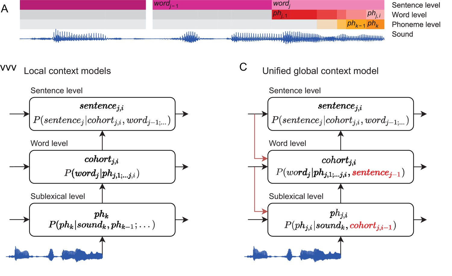
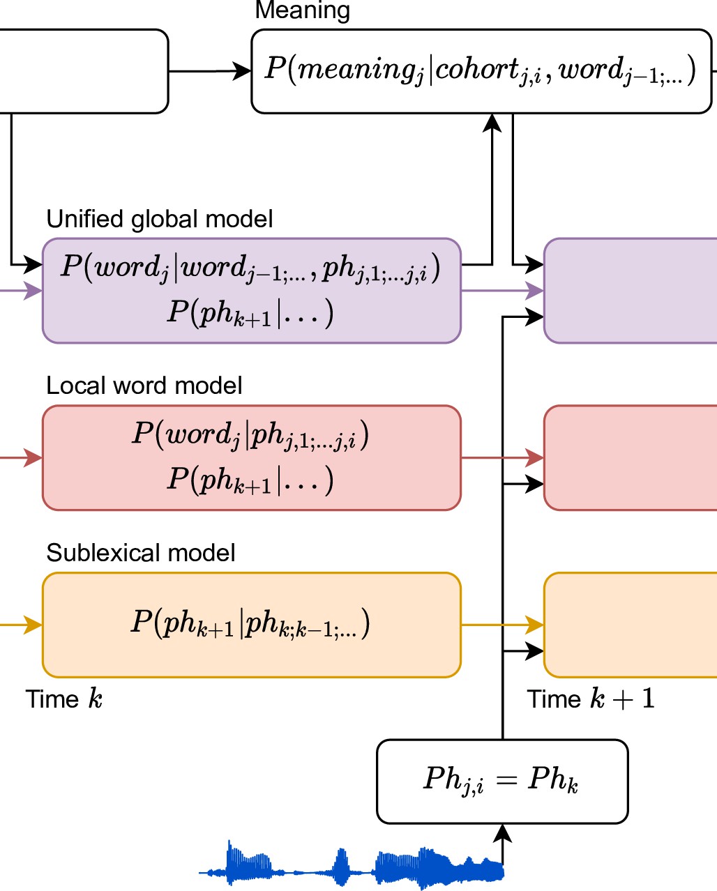
Information flow in local and unified architectures for speech processing.
(A) Schematic characterization of the linguistic units used to characterize speech. The same phoneme can be invoked as part of a sublexical phoneme sequence, phk, or as part of wordj, phj,i. (B) Each box stands for a level of representation, characterized by its output and a probability distribution describing the level’s use of context. For example, the sublexical level’s output is an estimate of the current phoneme, phk, and the distribution for phk is estimated as probability for different phonemes based on the sound input and a sublexical phoneme history. At the sentence level, sentencej,i stands for a temporary representation of the sentence at time j,i. Boxes represent functional organization rather than specific brain regions. Arrows reflect the flow of information: each level of representation is updated incrementally, combining information from the same level at the previous time step (horizontal arrows) and the level below (bottom-up arrows). (C) The unified architecture implements a unified, global context model through information flowing down the hierarchy, such that expectations at lower levels incorporate information accumulated at the sentence level. Relevant differences from the local context model are in red. Note that while the arrows only cross one level at a time, the information is propagated in steps and eventually crosses all levels.
Figure 2
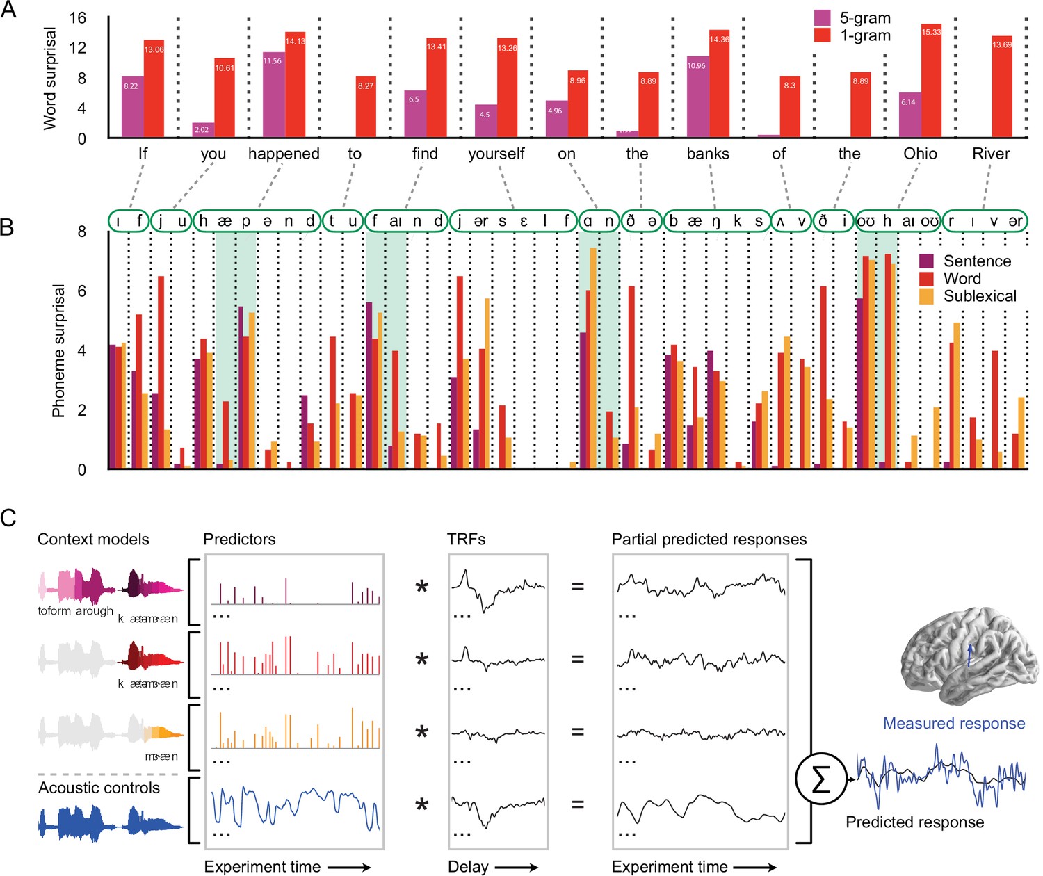
Models for predictive speech processing based on the sentence, word, and sublexical context, used to predict magnetoencephalography (MEG) data.
(A) Example of word-by-word surprisal. The sentence (5 gram) context generally leads to a reduction of word surprisal, but the magnitude of the reduction differs substantially between words (across all stimuli, mean ± standard deviation, unigram surprisal: 10.76 ± 5.15; 5 gram surprisal: 7.43 ± 5.98; t8172 = 76.63, p < 0.001). (B) Sentence-level predictions propagate to phoneme surprisal, but not in a linear fashion. For example, in the word happened, the phoneme surprisal based on all three models is relatively low for the second phoneme /æ/ due to the high likelihood of word candidates like have and had. However, the next phoneme is /p/ and phoneme surprisal is high across all three models. On the other hand, for words like find, on, and Ohio, the sentence-constrained phoneme surprisal is disproportionately low for subsequent phonemes, reflecting successful combination of the sentence constraint with the first phoneme. (C) Phoneme-by-phoneme estimates of information processing demands, based on different context models, were used to predict MEG responses through multivariate temporal response functions (mTRFs) (Brodbeck et al., 2018b). An mTRF consists of multiple TRFs estimated jointly such that each predictor, convolved with the corresponding TRF, predicts a partial response, and the pointwise sum of partial responses constitutes the predicted MEG response. The dependent measure (measured response) was the fixed orientation, distributed minimum norm source current estimate of the continuous MEG response. The blue arrow illustrates a single virtual current source dipole. Estimated signals at current dipoles across the brain were analyzed using a mass-univariate approach. See Methods for details. TRFs: temporal response functions.
Figure 3
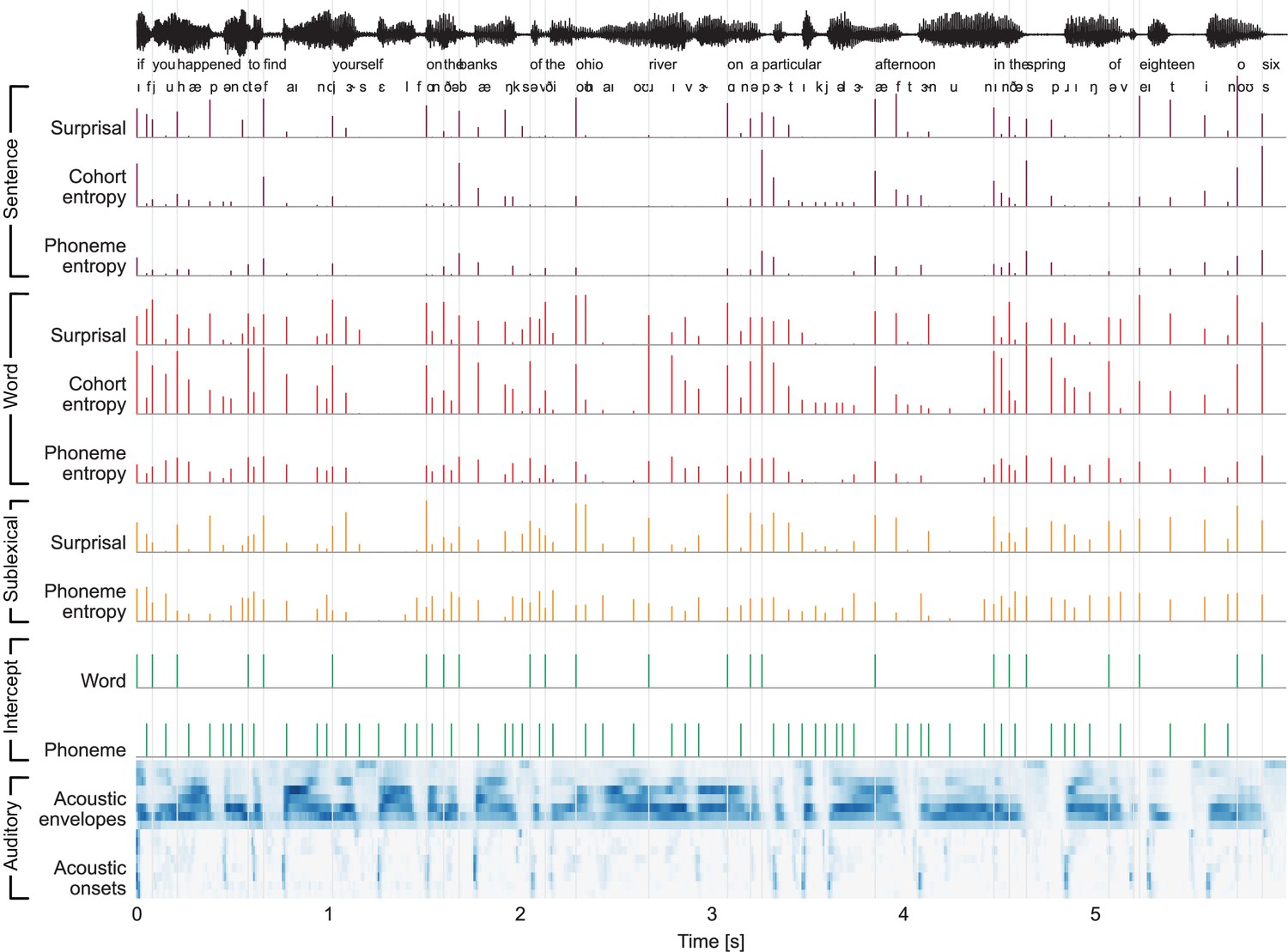
Stimulus excerpt with all 26 predictors used to model brain responses.
From the top: phoneme-level information-theoretic variables, based on different context definitions: sentence, word, and sublexical context; intercepts for word- and phoneme-related brain activity, that is, a predictor to control for brain activity that does not scale with the variables under consideration; and an auditory processing model, consisting of an acoustic spectrogram (sound envelopes) and an onset spectrogram (sound onsets), each represented by eight predictors for eight frequency bands.
Figure 4
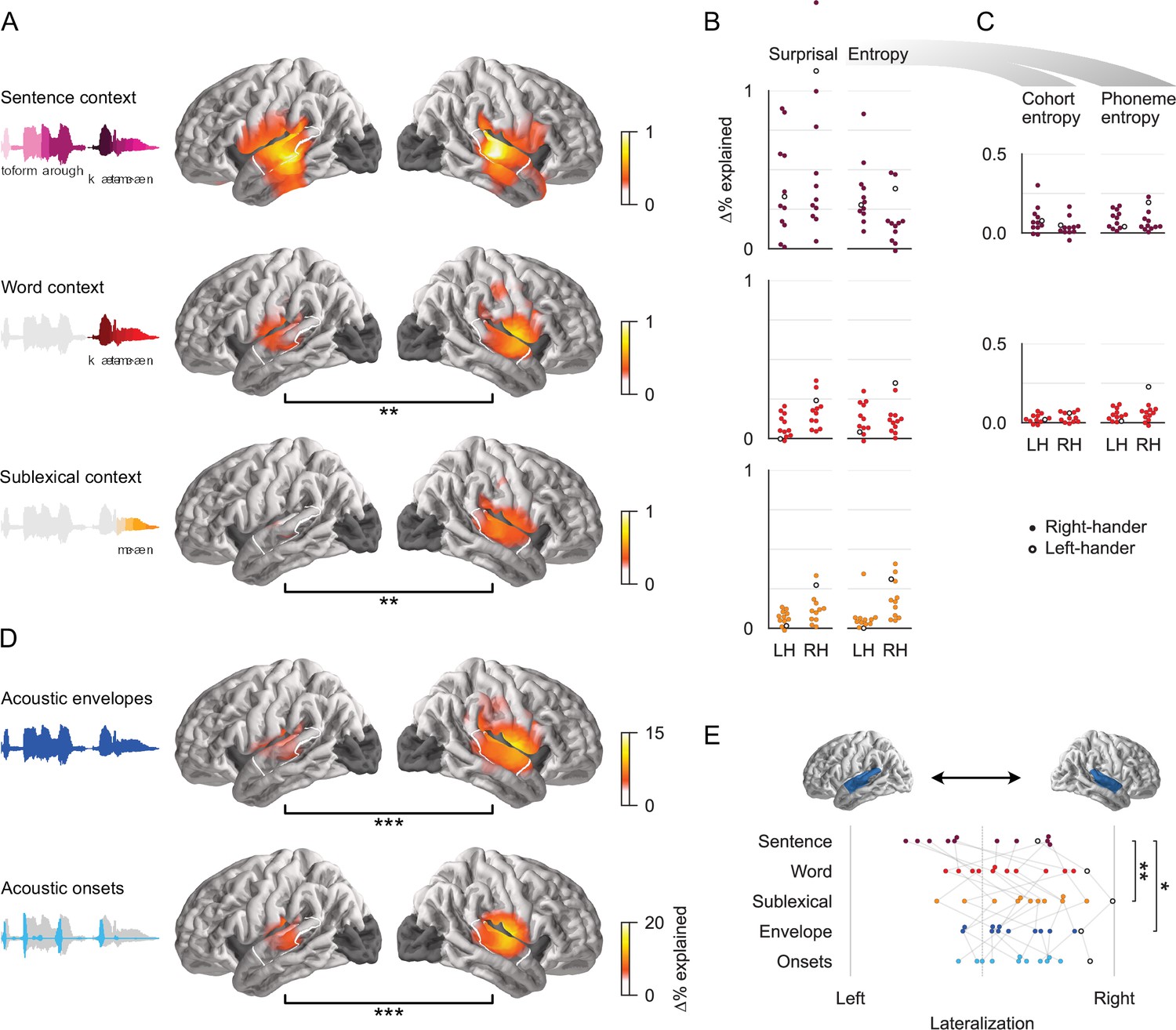
All context models significantly contribute to predictions of brain responses.
(A) Each context model significantly improves predictions of held-out magnetoencephalography (MEG) data in both hemispheres (tmax ≥ 6.16, p ≤ 0.005). Black bars below anatomical plots indicate a significant difference between hemispheres. The white outline indicates a region of interest (ROI) used for measures shown in (B), (C), and (E). Brain regions excluded from analysis are darkened (occipital lobe and insula). (B) Surprisal and entropy have similar predictive power in each context model. Each dot represents the difference in predictive power between the full and a reduced model for one subject, averaged in the ROI. Cohort- and phoneme entropy are combined here because the predictors are highly correlated and hence share a large portion of their explanatory power. Corresponding statistics and effect size are given in Table 1. A single left-handed participant is highlighted throughout with an unfilled circle. LH: left hemisphere; RH: right hemisphere. (C) Even when tested individually, excluding variability that is shared between the two, cohort- and phoneme entropy at each level significantly improve predictions. A significant effect of sentence-constrained phoneme entropy is evidence for cross-hierarchy integration, as it suggests that sentence-level information is used to predict upcoming phonemes. (D) Predictive power of the acoustic feature representations. (E) The lateralization index indicates that the sublexical context model is more right-lateralized than the sentence context model. Left: LI = 0; right: LI = 1. Significance levels: *p ≤ 0.05; **p ≤ 0.01; ***p ≤ 0.001.
-
Figure 4—source data 1
Mass-univariate statistics results for Panels A & D.
- https://cdn.elifesciences.org/articles/72056/elife-72056-fig4-data1-v2.zip
-
Figure 4—source data 2
Predictive power in the mid/posterior superior temporal gyrus ROI, data used in Panels B, C & E.
- https://cdn.elifesciences.org/articles/72056/elife-72056-fig4-data2-v2.zip
Figure 5
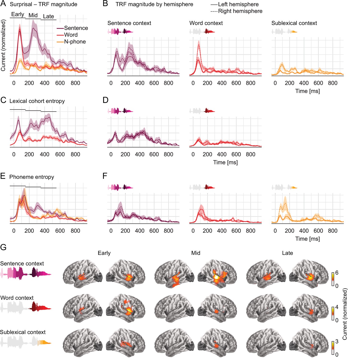
Early responses reflect parallel activation of all context models, later responses selectively reflect activity in the sentence-constrained model.
(A) Current magnitude of temporal response functions (TRFs) to phoneme surprisal for each level of context (mean and within-subject standard error [Loftus and Masson, 1994]; y-axis scale identical in all panels of the figure). To allow fair comparison, all TRFs shown are from the same symmetric region of interest, including all current dipoles for which at least one of the three context models significantly improved the response predictions. Bars indicate time windows corresponding to source localizations shown in panel G. (B) When plotted separately for each hemisphere, relative lateralization of the TRFs is consistent with the lateralization of predictive power (Figure 4). (C, D) TRFs to lexical cohort entropy are dominated by the sentence context model. (E, F) TRFs to phoneme entropy are similar between context models, consistent with parallel use of different contexts in predictive models for upcoming speech. (G) All context models engage the superior temporal gyrus at early responses, midlatency responses incorporating the sentence context also engage more ventral temporal areas. Anatomical plots reflect total current magnitude associated with different levels of context representing early (−50 to 150 ms), midlatency (150–350 ms), and late (350–550 ms) responses. The color scale is adjusted for different predictors to avoid images dominated by the spatial dispersion characteristic of magnetoencephalography source estimates.
-
Figure 5—source data 1
Temporal response function peak latencies in the early time window.
- https://cdn.elifesciences.org/articles/72056/elife-72056-fig5-data1-v2.zip
-
Figure 5—source data 2
Pairwise tests of temporal response function time courses.
- https://cdn.elifesciences.org/articles/72056/elife-72056-fig5-data2-v2.zip
Figure 6
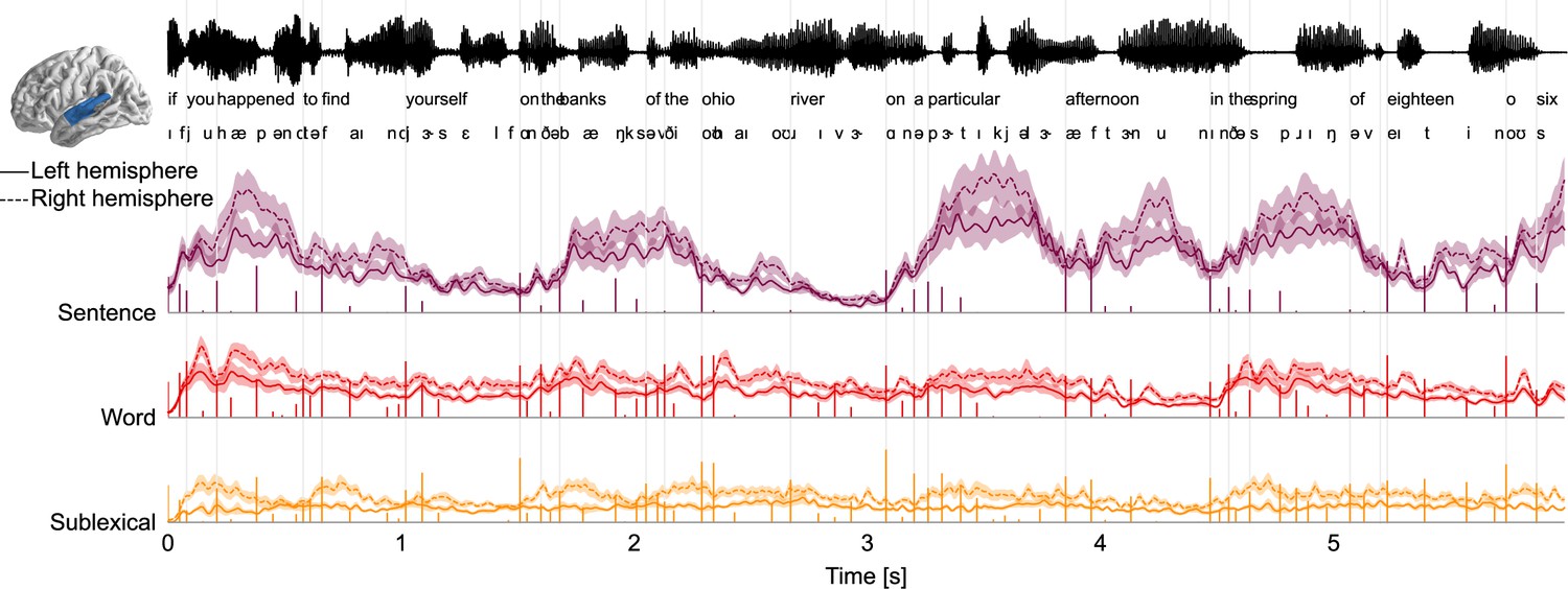
Decomposition of brain responses into context levels.
Predicted brain responses related to processing different levels of context (combining surprisal and entropy predictors; mean and within-subject standard error). Stem plots correspond to surprisal for the given level. Slow fluctuations in brain responses are dominated by the sentence level, with responses occurring several hundred milliseconds after surprising phonemes, consistent with the high amplitude at late latencies in temporal response functions (TRFs). Partial predicted responses were generated for each context model by convolving the TRFs with the corresponding predictors; summing the predicted responses for the predictors corresponding to the same level; and extracting the magnitude (sum of absolute values) in the superior temporal gyrus region of interest.
Figure 7
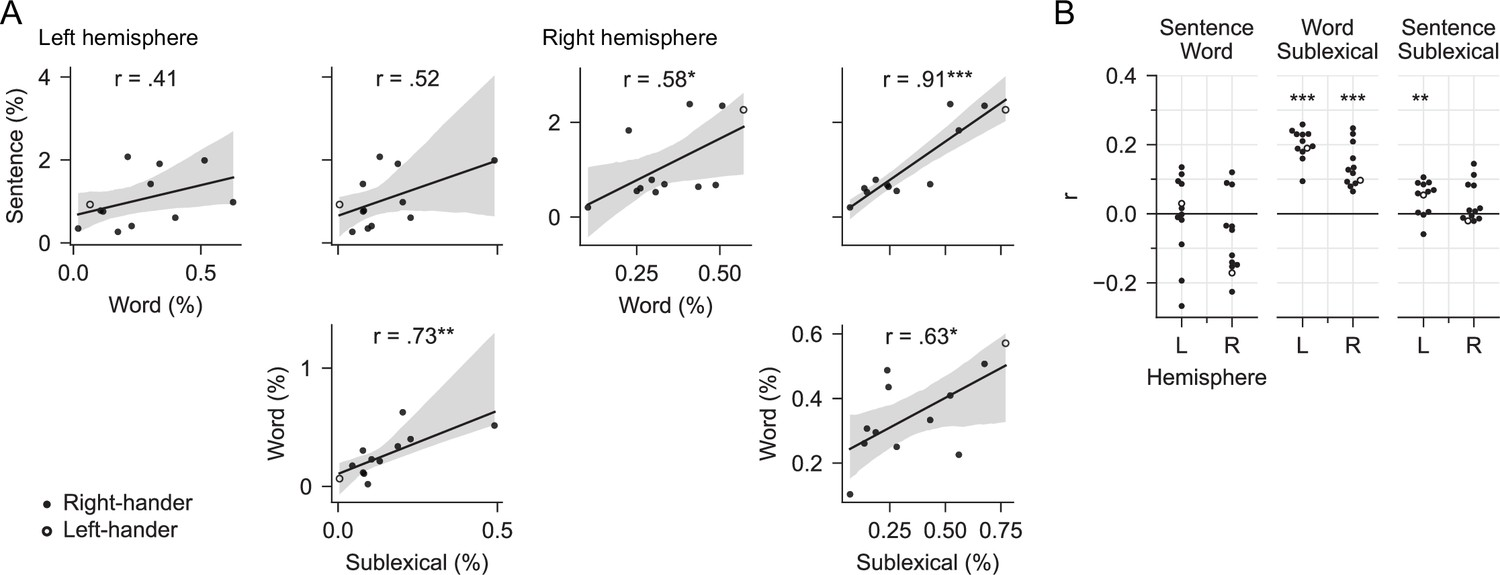
No evidence for a trade-off between context models.
(A) Trade-off across subjects: testing the hypothesis that subjects differ in which context model they rely on. Each plot compares the predictive power of two context models in the mid/posterior superior temporal gyrus region of interest, each dot representing % explained for one subject. The line represents a linear regression with 95% bootstrap confidence interval (Waskom, 2021). None of the pairwise comparisons exhibits a negative correlation that would be evidence for a trade-off between reliance on different context models. Data from Figure 4—source data 2. (B) Trade-off over time: testing the hypothesis that subjects alternate over time in which context model they rely on. Each dot represents the partial correlation over time between the predictive power of two context models for one subject, controlling for predictive power of the full model. Correlations are shown separately for the left and the right hemisphere (L/R). Stars correspond to a one-sample t-tests of the null hypothesis that the average r across subjects is 0, that is, that the two context models are unrelated over time. None of the context models exhibited a significant negative correlation that would be evidence for a trade-off over time.
-
Figure 7—source data 1
Partial correlations over time for each subject (data for Panel B).
- https://cdn.elifesciences.org/articles/72056/elife-72056-fig7-data1-v2.zip
Figure 8
An architecture for speech perception with multiple parallel context models.
A model of information flow, consistent with brain signals reported here. Brain responses associated with Information-theoretic variables provide separate evidence for each of the probability distributions in the colored boxes. From left to right, the three different context models (sentence, word, and sublexical) update incrementally as each phoneme arrives. The cost of these updates is reflected in the brain response related to surprisal. Representations also include probabilistic representations of words and upcoming phonemes, reflected in brain responses related to entropy.
Tables
Table 1
Predictive power in mid/posterior superior temporal gyrus region of interest for individual predictors.
One-tailed t-tests and Cohen’s d for the predictive power uniquely attributable to the respective predictors. Data underlying these values are the same as for the swarm plots in Figure 4B, C (Figure 4—source data 2). *p ≤ 0.05; **p ≤ 0.01; ***p ≤ 0.001.
| Left hemisphere | Right hemisphere | ||||||||
|---|---|---|---|---|---|---|---|---|---|
| ∆‰ | t(11) | p | d | ∆‰ | t(11) | p | d | ||
| Sentence context | |||||||||
| Surprisal | 3.77 | 4.40** | 0.001 | 1.27 | 5.51 | 4.14** | 0.002 | 1.19 | |
| Entropy | 3.40 | 5.96*** | <0.001 | 1.72 | 1.94 | 4.11** | 0.002 | 1.19 | |
| Cohort | 0.83 | 3.41** | 0.006 | 0.98 | 0.39 | 2.45* | 0.032 | 0.71 | |
| Phoneme | 0.85 | 5.18*** | <0.001 | 1.50 | 0.79 | 3.85** | 0.003 | 1.11 | |
| Word context | |||||||||
| Surprisal | 0.78 | 3.62** | 0.004 | 1.04 | 1.71 | 5.76*** | <0.001 | 1.66 | |
| Entropy | 1.26 | 4.43** | 0.001 | 1.28 | 1.31 | 4.39** | 0.001 | 1.27 | |
| Cohort | 0.25 | 3.29** | 0.007 | 0.95 | 0.36 | 3.99** | 0.002 | 1.15 | |
| Phoneme | 0.51 | 4.59*** | <0.001 | 1.32 | 0.66 | 3.61** | 0.004 | 1.04 | |
| Sublexical context | |||||||||
| Surprisal | 0.64 | 4.88*** | <0.001 | 1.41 | 1.29 | 4.59*** | <0.001 | 1.33 | |
| Entropy | 0.66 | 2.53* | 0.028 | 0.73 | 1.91 | 5.32*** | <0.001 | 1.54 | |
Additional files
Download links
A two-part list of links to download the article, or parts of the article, in various formats.
Downloads (link to download the article as PDF)
Open citations (links to open the citations from this article in various online reference manager services)
Cite this article (links to download the citations from this article in formats compatible with various reference manager tools)
Parallel processing in speech perception with local and global representations of linguistic context
eLife 11:e72056.
https://doi.org/10.7554/eLife.72056


