Mechanisms of distributed working memory in a large-scale network of macaque neocortex
- Swammerdam Institute for Life Sciences, University of Amsterdam, Netherlands
- Center for Neural Science, New York University, United States
Figures
Figure 1 with 2 supplements

Scheme and anatomical basis of the multi-regional macaque neocortex model.
(A) Lateral view of the macaque cortical surface with modelled areas in color. (B) In the model, inter-areal connections are calibrated by mesoscopic connectomic data (Markov et al., 2013), each parcellated area is modeled by a population firing rate description with two selective excitatory neural pools and an inhibitory neural pool (Wong and Wang, 2006). Recurrent excitation within each selective pool is not shown for the sake of clarity of the figure. (C) Correlation between spine count data (Elston, 2007) and anatomical hierarchy as defined by layer-dependent connections (Markov et al., 2014a).
Figure 1—figure supplement 1
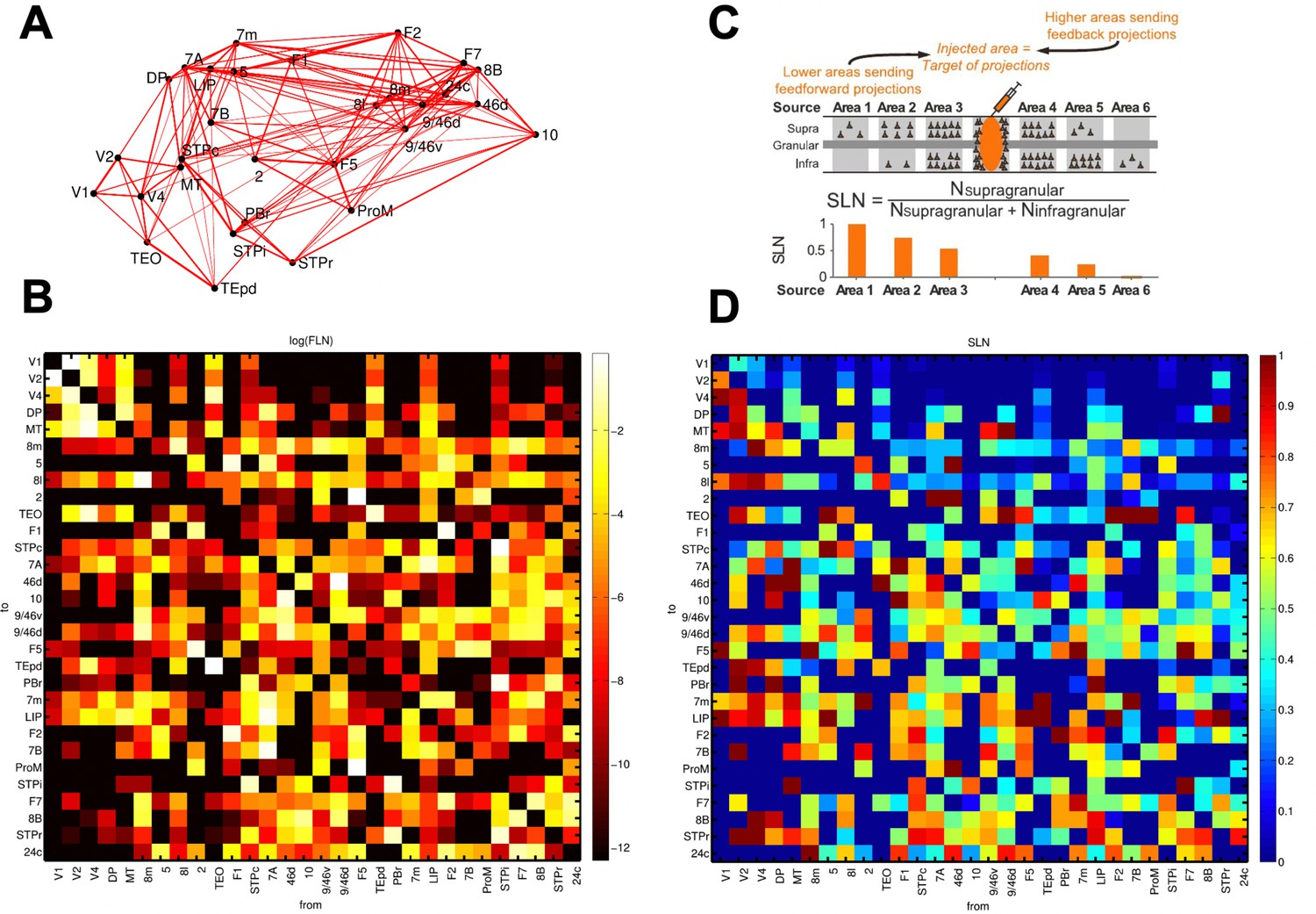
Anatomical connectivity data of the macaque cortex.
Data from anatomical studies (Markov et al., 2013; Markov et al., 2014a; Markov et al., 2014b). (A) Connectivity of the 30 areas (positioned in 3D space following injection coordinates of experiments). Width of the lines denote two-way averaged FLN values (i.e. average strength of the projection). (B) Map of FLN values for all connections considered. (C) The proportion of supragranular vs infragranular neurons projecting to the injection site allowed to define an anatomical hierarchy. (D) Map of SLN values for all connections considered.
Figure 1—figure supplement 2
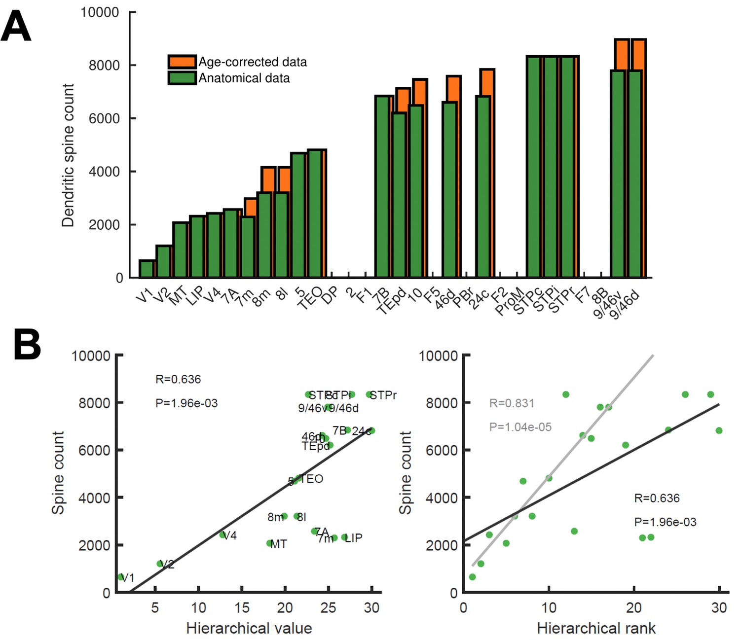
Spine count data used to constrain connectivity strength.
Data from anatomical studies (Elston, 2007), see also Table 1. (A) Spine count of the basal dendrites of layer 2/3 neurons across cortical areas of young (2~3years old) macaques. When data from older macaques had to be considered, an age correction was introduced (orange bars). (B) Correlation between the spine count data and the hierarchical value hi (left) or the hierarchical position/rank (right). A robust fit obtained by random sampling consensus (grey, 100 randomized trials with a threshold for number of outliers < 10% of the total points) suggest areas 7m and LIP as potential outliers. Pearson correlation and corresponding p-value are shown in each panel. In the model, the connectivity strength of areas for which spine count data was not available was estimated using their hierarchical value.
Figure 2 with 5 supplements
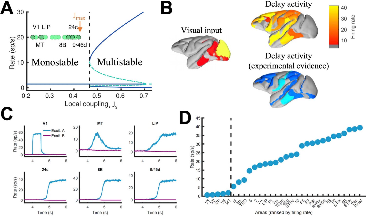
Distributed WM sustained via long-range loops in cortical networks.
(A) Bifurcation diagram for an isolated area. Green circles denote the position of each area, with all of them in the monostable regime when isolated. (B) Spatial activity map during visual stimulation (left) and delay period (upper right). For comparison purposes, bottom right map summarizes the experimental evidence of WM-related delay activity across multiple studies (Leavitt et al., 2017), dark blue corresponds to strong evidence and light blue to moderate evidence. (C) Activity of selected cortical areas during the WM task, with a selective visual input of 500ms duration. (D) Firing rate for all areas during the delay period, ranked by firing rate.
Figure 2—figure supplement 1
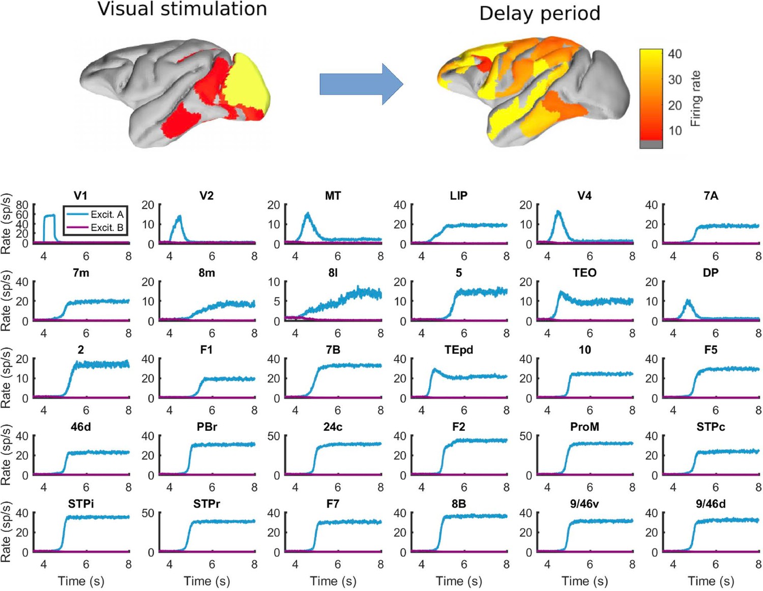
Behavior of all areas in the network during the visual WM task.
Top: spatial maps of the simulated macaque brain during stimulation and delay period, with activity color coded. Bottom: evolution of the firing rate of all areas in the network. Stimulation occurs in V1 at t = 4 s and has a duration of 500ms. Parameters as in Figure 2.
Figure 2—figure supplement 2
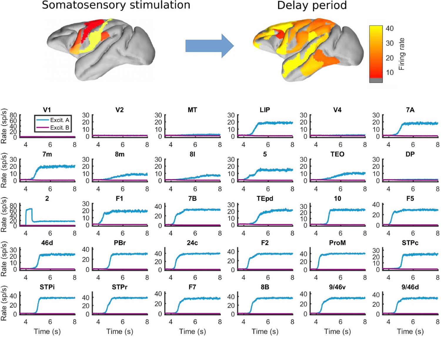
Behavior of all areas in the network during the somatosensory WM task.
Top: spatial maps of the simulated macaque brain during stimulation and delay period, with activity color coded. Bottom: evolution of the firing rate of all areas in the network. Stimulation occurs in area 2 (primary somatosensory area) at t = 4 seconds, and has a duration of 500ms. Other parameters as in Figure 2.
Figure 2—figure supplement 3

A simple gating mechanism controls the participation of areas in distributed WM.
(A) Response of all cortical areas when gates are closed for all areas (orange), open for visual areas only (green) and open to all areas (blue). Note that areas not involved in visual processing, such as somatosensory areas, are not activated by the input when only visual areas are gated. (B) Spatial activity maps for the delay period corresponding to the three cases in panel A. A weak global coupling (G = 0.2) is used to provide room for the effects of gating (see Materials and Methods), all other parameters as in Figure 2. For the purposes of the gating simulation, ‘visual’ areas were selected according to a recent meta-analysis: V1, V2, V4, MT, LIP, 7a, TEO, TEpd, 8l, 8m, 8B, 46d, 9/46d, and 9/46v. The strength of the gating modulation is gs = 0.38 for the visual-only case, and gs = 0.28 for the all-areas case since it involves more areas (this situation is roughly equivalent to Figure 2).
Figure 2—figure supplement 4

Firing rates for selected areas during a visual WM task with a short (50ms) stimulus duration.
(A) Only NMDA and GABA synapses are considered in the network, the stimulus does not reach frontal areas. (B) By introducing simplified AMPA-like synapses (proportional to the firing rates) on feedforward excitatory projections, we obtain distributed WM patterns for this type of short inputs. The results suggests that it is convenient to consider AMPA/NMDA asymmetry along the FF/FB projections in the hierarchy for brief stimulation patterns. Other parameters as in Figure 2.
Figure 2—figure supplement 5

Firing rate of ranked cortical areas reveals a robust transition in space with different ranking systems.
(A) Areas ranked by displayed firing rate. (B) Areas ranked by spine count. (C) Areas ranked following their hierarchical (as obtained from SLN data) position. Parameters as in Figure 2.
Figure 3 with 1 supplement
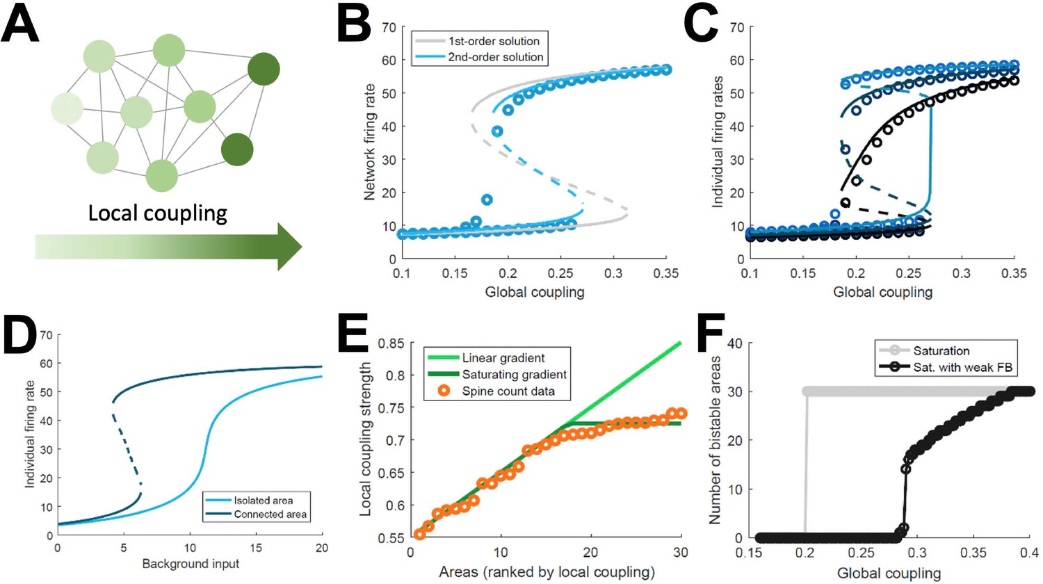
Simplified model of distributed WM.
(A) Scheme of our simplified model: a fully connected network of N = 30 excitatory nodes with a gradient of local coupling strength. (B) Population-average firing rate as a function of the global coupling strength, according to numerical simulations (symbols) and a mean-field solution based on first-order (gray line) or second-order statistics (blue). (C) Firing rates of three example individual nodes (symbols denote simulations, lines denote second-order mean-field solutions). (D) Activity of an example node when isolated (light blue) or connected to the network (dark blue). (E) Two forms for the gradient of local coupling strength (lines) compared with the spine count data (symbols). (F) The number of bistable areas in the attractor (grey) is either zero or N when the gradient of local properties saturates as suggested by spine count data. When feedback projections become weaker, resembling inhibitory feedback, the network is able to display distributed WM patterns which involve only a limited number of areas (black).
Figure 3—figure supplement 1
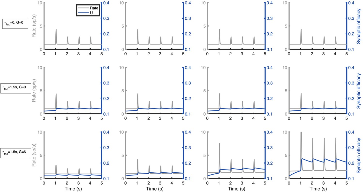
Simplified network model for distributed, activity-silent memory traces.
We modified our simplified network model (see Figure 3) to incorporate short-term synaptic facilitation (STF) in its local and long-range projections (see Materials and methods). Original projection strengths were reduced from the original values to allow STF to enhance synaptic strengths in an activity-dependent manner. Columns show traces of firing rate and synaptic efficacy (resp. baseline of P) for areas from the bottom (left) to the top (right) section of the linear gradient of local strengths. Top row: network without STF and isolated areas. Middle row: network with STF (time constant of 1.5 s) and isolated areas. Bottom row: network with STF (time constant of 1.5 s) and interconnected areas (G = 6). Parameters are P = 0.1 (initial synaptic probability release), background current I=-10, η1 = 0.05, ηN=0.25, δ = 0.05. External input are pulses of 50ms duration arriving every second at the lowest area of the linear gradient (simulating a primary sensory area), the first pulse has a strength of 15 and the rest (internal ‘ping’ signals) of 10. Other parameters as in Figure 3 B.
Figure 4 with 3 supplements
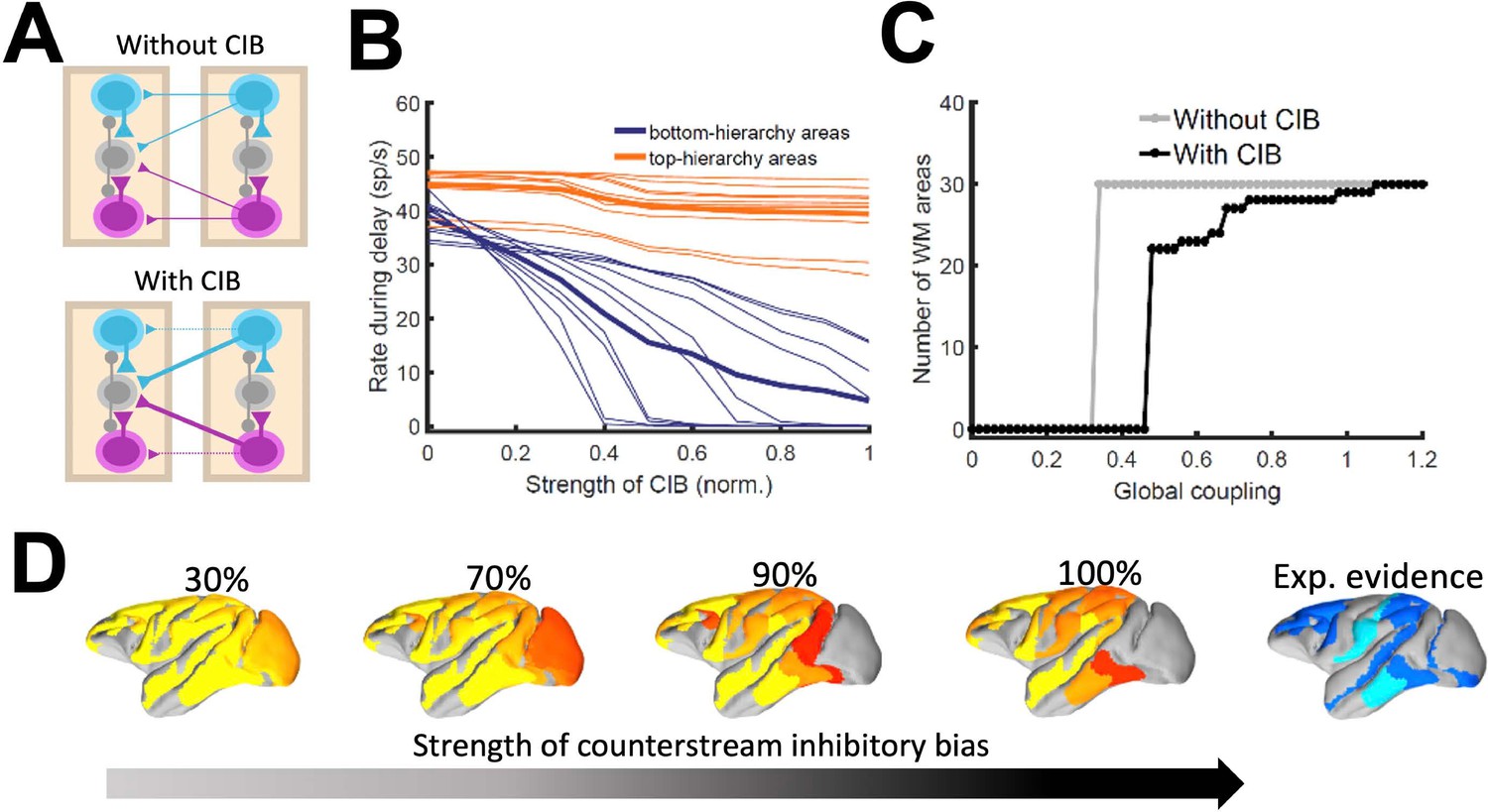
Effect of inhibitory feedback on distributed WM for the full model.
(A) Scheme showing a circuit without (left) or with (right) the assumption of counterstream inhibitory bias, or CIB. (B) Firing rate of areas at the bottom and top of the hierarchy (10 areas each, thick lines denote averages) as a function of the CIB strength. (C) Number of areas showing sustained activity in the example distributed activity pattern vs global coupling strength without (grey) and with (black) CIB. (D) Activity maps as a function of the CIB strength. As in Figure 2 B, bottom map denotes the experimental evidence for each area (dark blue denotes strong evidence, light blue denotes moderate evidence).
Figure 4—figure supplement 1
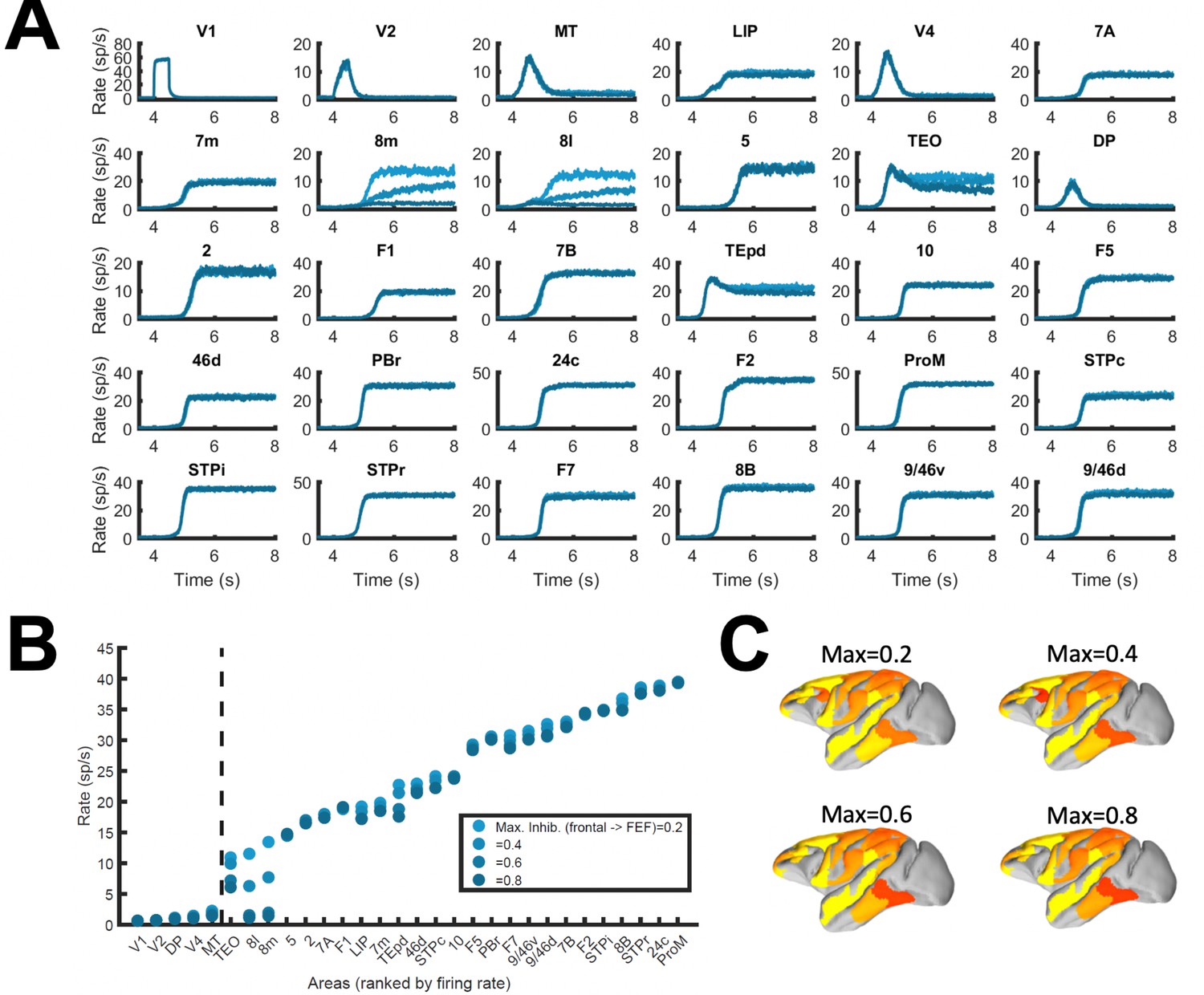
Corrections to localized regions; example of FEF areas.
(A) Traces of every area in the simulated neocortical network. We limit here the strength of counterstream inhibitory bias, or preference of feedback towards inhibition, which feedback projections from frontal areas to FEF areas (8 l and 8 m) may display. For each plotted area, blue lines of increasing darkness show the effects of limiting frontal inhibitory feedback to FEF to 0.2, 0.4, 0.6, or 0.8. The effects are mostly visible in areas 8 l and 8 m, and to a lesser extent in TEO. (B) Transition in the cortical space for the different limitations to FEF inhibitory feedback. (C) Activity maps for the four conditions shown in panels A and B. Other parameters as in Figure 2.
Figure 4—figure supplement 2
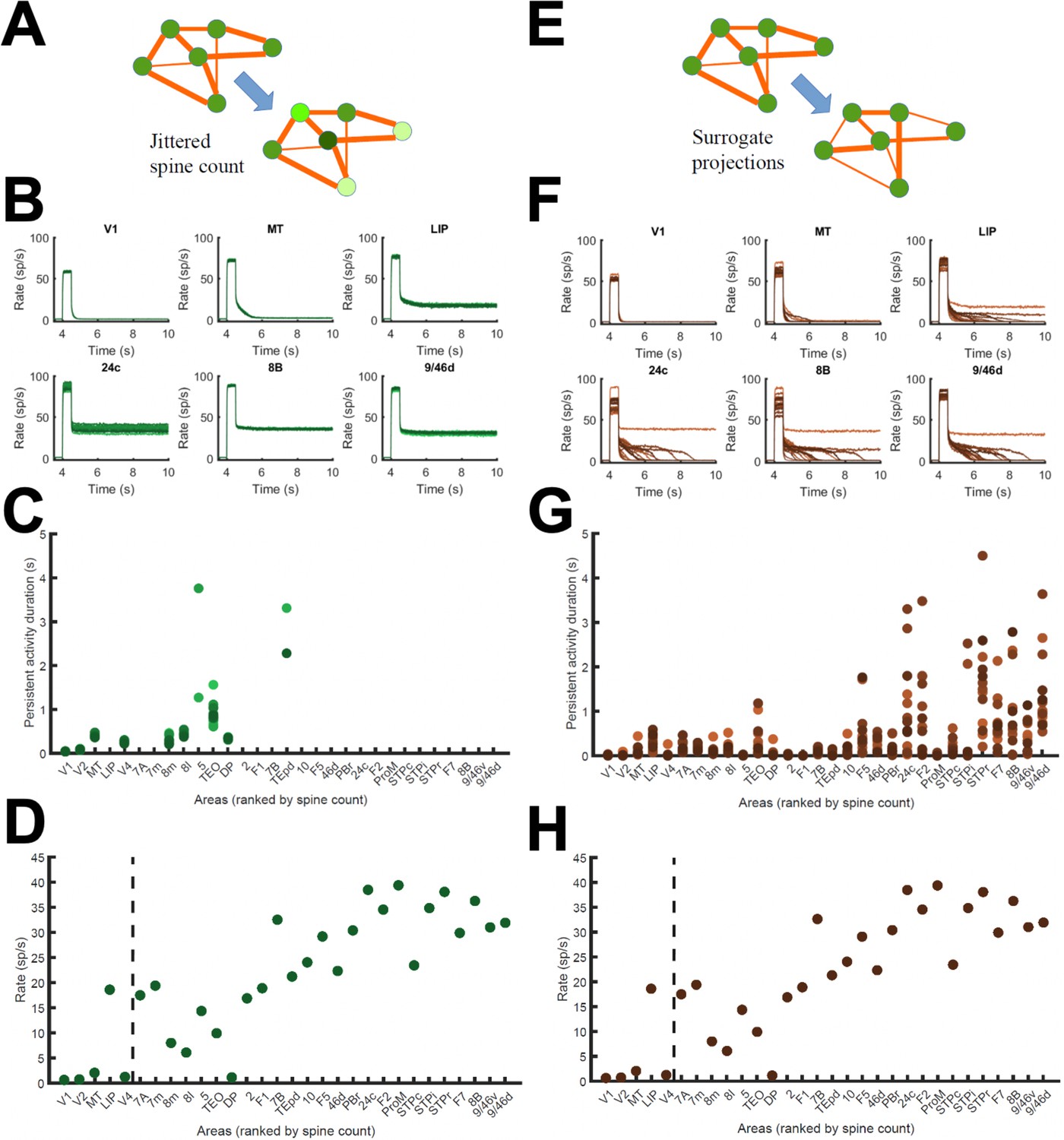
Effect of jitter on dendritic spine values and surrogate networks.
(A) Scheme of networks with jittered area-specific dendritic spine numbers (within 15% of their original values), and therefore jittered local and long-range synaptic strengths. (B) Effects of the jitter in traces for selected areas (lines of different colors represent activity for different configurations). (C) Jittering has a minor effect on the duration of the sustained state for low/middle spine count areas. (D) Transition in cortical space for jittered networks. (E) Scheme of surrogate networks, in which FLN values are randomly shuffled. (F) Effects of shuffling FLN values on traces of selected areas. (G) Surrogate networks present moderate differences in the duration of the sustained states of high spine count values. (H) Transition in cortical space for surrogate networks. Parameters as in Figure 2.
Figure 4—figure supplement 3

A gradient of time scales emerges in the network.
(A) Autocorrelation function of the activity (low-pass-filtered to simulate an LFP recording) of each area in the network, fitted with a decaying exponential function. (B) The values for the local decay time constant increase with the cortical hierarchy, going from ~60 ms in early visual areas to ~300 ms in some frontal areas. This range is similar to the spike-count autocorrelations found experimentally across different cortical areas (Murray et al., 2014; Siegle, 2019), and improves predictions from previous models (Chaudhuri et al., 2015) but see additional considerations Schmidt et al., 2018. Parameters as in Figure 2.
Figure 5
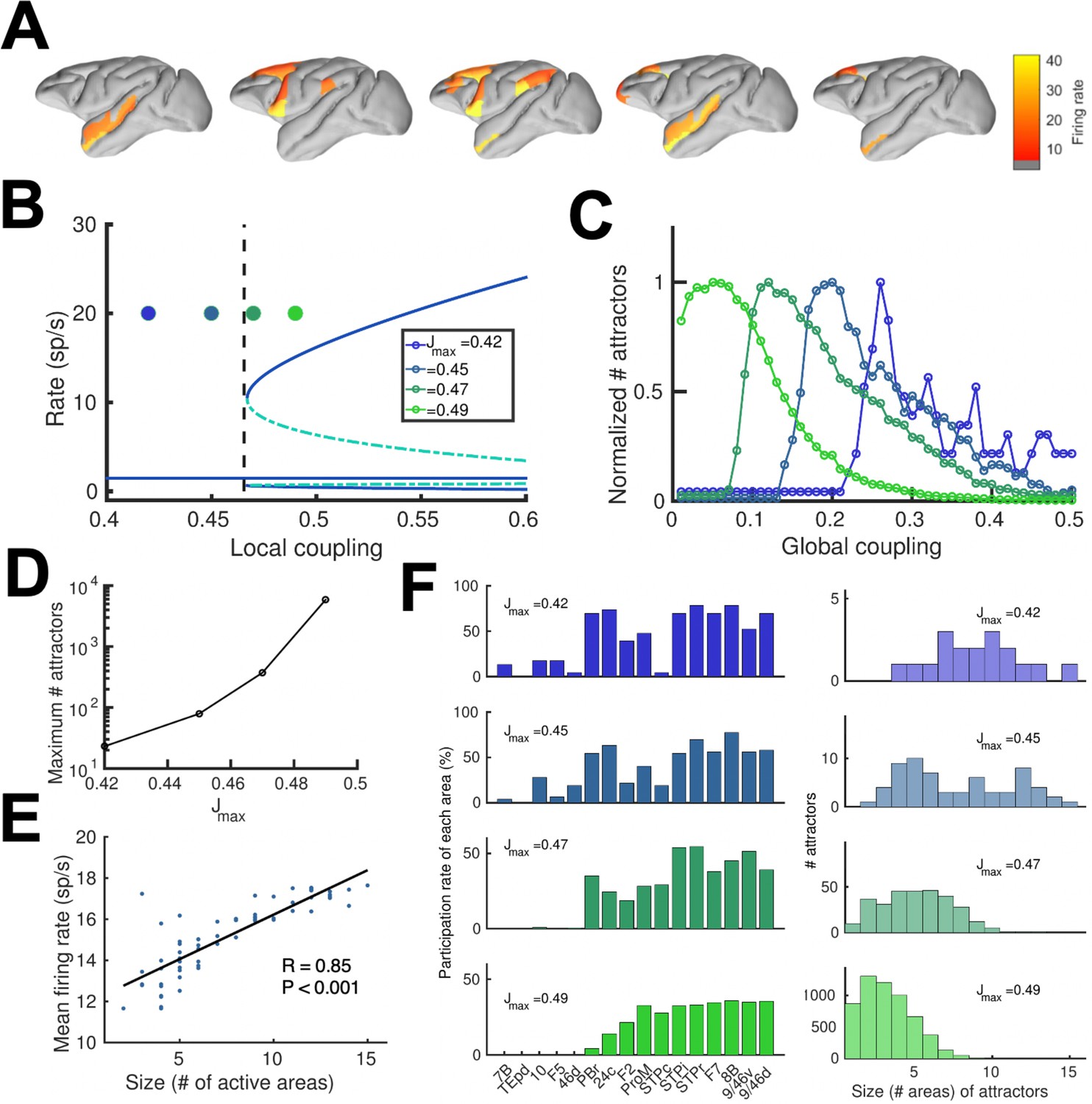
Distributed and local WM mechanisms can coexist in the full model.
(A) Five example distributed attractors of the network model (Jmax = 0.42). (B) Bifurcation diagram of an isolated local area with the four cases considered. (C) Number of attractors (normalized) found via numerical exploration as a function of the global coupling for all four cases. (D) Maximum (peak) number of attractors for each one of the cases. (E) Correlation between size of attractors and mean firing rate of its constituting areas for Jmax = 0.45and G = 0.2. (F) Participation index of each area (left, arranged by spine count) and distribution of attractors according to their size (right).
Figure 6
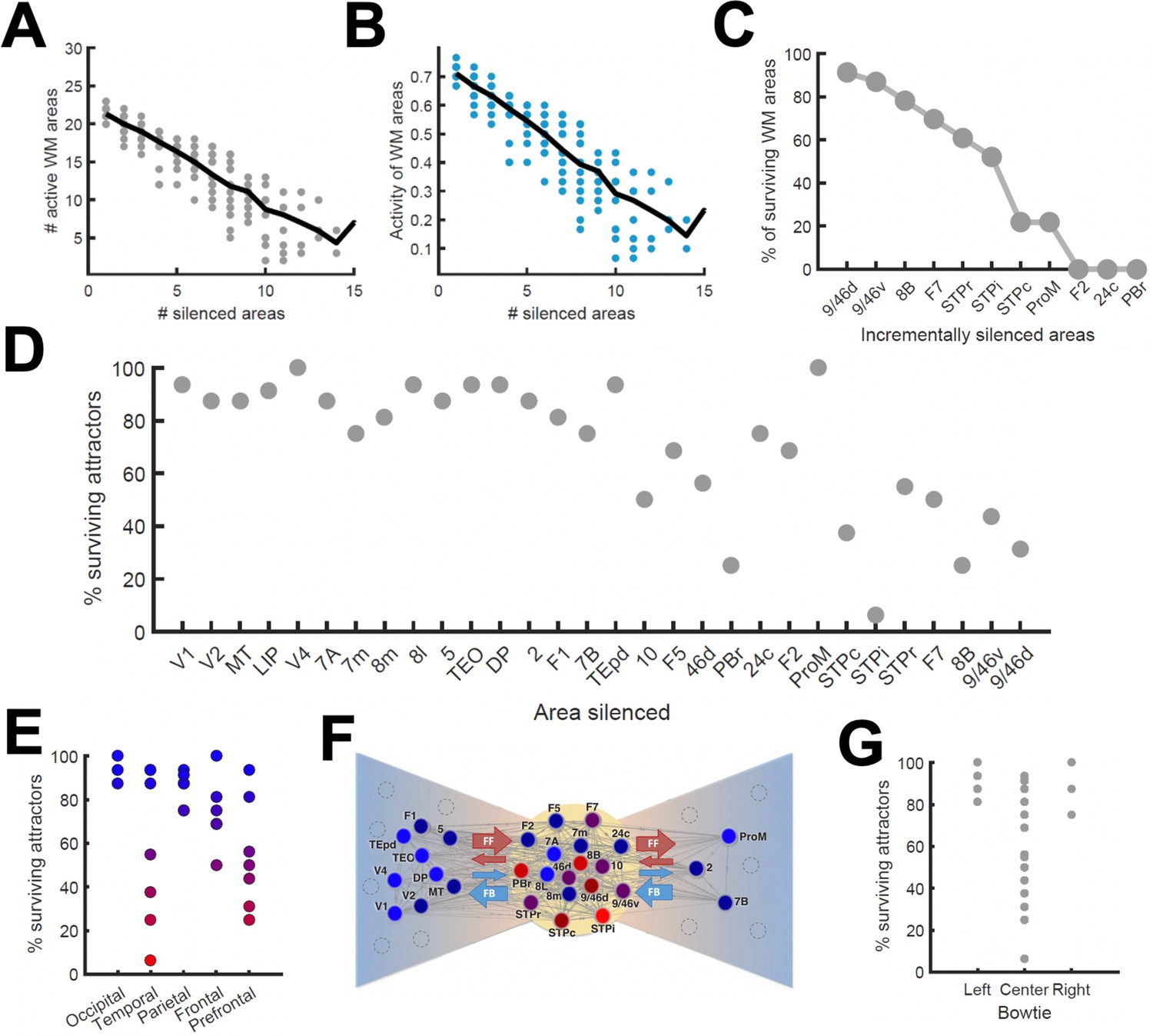
Effects of lesioning/silencing areas on the activity and number of attractors.
Silencing occurs throughout the full trial for each area indicated here. (A) Number of active areas in the example attractor as a function of the number of (randomly selected) silenced areas. (B) The activity of the areas which remain as part of the attractor decreases with the number of silenced areas. (C) The number of active WM areas decreases faster when areas are incrementally and simultaneously silenced in reverse hierarchical order. (D) When considering all accessible attractors for a given network (G = 0.48, Jmax = 0.42), silencing areas at the top of the hierarchy has a higher impact on the number of surviving attractors than silencing bottom or middle areas. (E) Numerical exploration of the percentage of surviving attractors for silencing areas in different lobes. (F) Silencing areas at the center of the ‘bowtie hub’ has a strong impact on WM (adapted from Markov et al., 2013). (G) Numerical impact of silencing areas in the center and sides of the bowtie on the number of surviving attractors. For panels (E) and (F), areas color-coded in blue/red have the least/most impact when silenced, respectively.
Figure 7
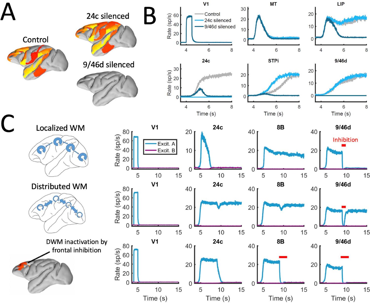
Effect of silencing areas in localized vs distributed WM.
(A) Full-brain activity maps during the delay period for the control case (left), and lesioning/silencing area 24 (top right) or area 9/46d (bottom right). (B) Traces of selected areas for the three cases in panel A show the effects of silencing each area. (C) For a network displaying localized WM (top row, corresponding to Jmax = 0.468, G = 0.21), a brief inactivation of area 9/46d leads to losing the selective information retained in that area. For a network displaying distributed working memory (middle row, Jmax = 0.26, G = 0.48) a brief inactivation removes the selective information only transiently, and once the external inhibition is removed the selective information is recovered. In spite of this robustness to brief inactivations, distributed WM patters can be shut down by inhibiting a selective group of frontal areas simultaneously (bottom row, inhibition to areas 9/46 v, 9/46d, F7, and 8B). The shut-down input, of strength I = 0.3 and 1s duration, is provided to the nonselective inhibitory population of each of these four areas.
Figure 8
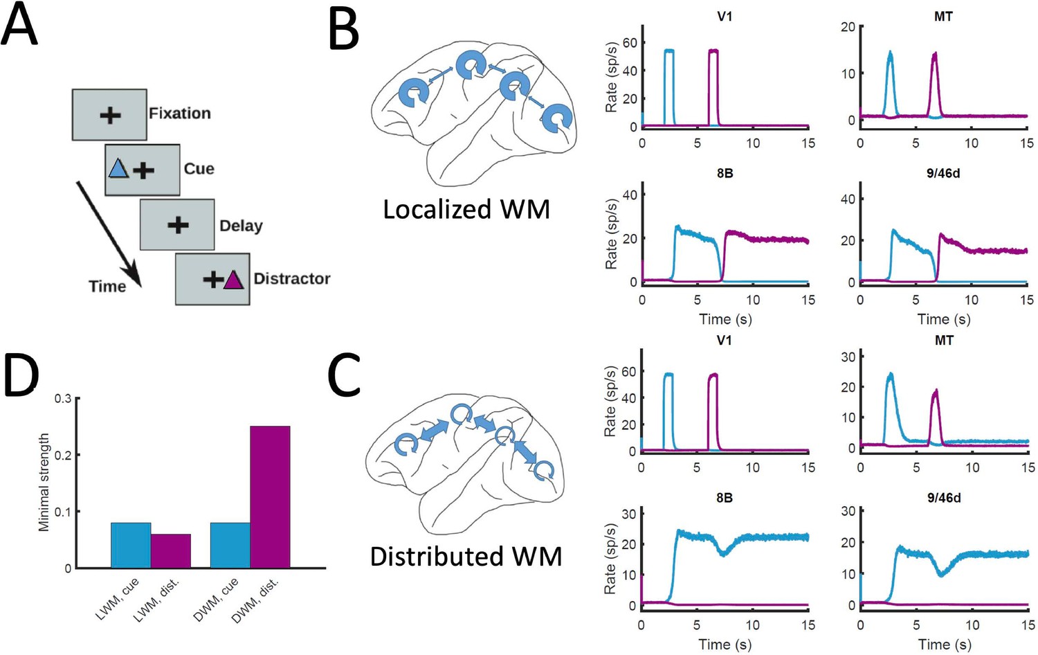
Resistance to distractors in localized vs distributed WM.
(A) Scheme of the WM task with a distractor, with the cue (current pulse of strength IA = 0.3 and duration 500ms) preceding the distractor (IB = 0.3, 500ms) by four seconds. (B) Activity traces of selected areas during the task, for a network displaying localized WM (Jmax = 0.468, G = 0.21). (C) Same as panel B, but for a model displaying distributed WM (Jmax = 0.26, G = 0.48). (D) Minimal strength required by the cue (blue) to elicit a sustained activity state, and minimal strength required by the distractor (purple) to remove the sustained activity, both for localized WM (left) and distributed WM (right).
Author response image 1
Tables
Table 1
Spine count data from basal dendrites of layer 2/3 pyramidal neurons in young (~2y o) macaque, acquired from the specified literature.
See also Figure 1—figure supplement 2.
| Rank in SLN hierarchy | Area name | Measured spine count | Age correction factor | Source |
|---|---|---|---|---|
| 1 | V1 | 643 | 1 | Elston et al., 1999; Elston and Rosa, 1997 |
| 2 | V2 | 1201 | 1 | Elston and Rosa, 1997 |
| 3 | V4 | 2429 | 1 | Elston and Rosa, 1998b |
| 4 | DP | - | - | |
| 5 | MT | 2077 | 1 | Elston et al., 1999 |
| 6 | 8m | 3200 | 1.30 | Elston and Rosa, 1998b |
| 7 | 5 | 4689 | 1 | Elston and Rockland, 2002 |
| 8 | 8l | 3200 | 1.30 | Elston and Rosa, 1998b |
| 9 | 2 | - | - | |
| 10 | TEO | 4812 | 1 | Elston and Rosa, 1998b |
| 11 | F1 | - | - | |
| 12 | STPc | 8337 | 1 | Elston et al., 1999 |
| 13 | 7a | 2572 | 1 | Elston and Rosa, 1997; Elston and Rosa, 1998a |
| 14 | 46d | 6600 | 1.15 | Estimated from Elston, 2007; |
| 15 | 10 | 6488 | 1.15 | Elston et al., 2011 |
| 16 | 9/46 v | 7800 | 1.15 | Estimated from Elston, 2007 |
| 17 | 9/46d | 7800 | 1.15 | Estimated from Elston, 2007 |
| 18 | F5 | - | - | |
| 19 | TEpd | 7260 | 1 | Elston et al., 1999 |
| 20 | PBr | - | - | |
| 21 | 7m | 2294 | 1.30 | Elston, 2001 |
| 22 | LIP | 2316 | 1 | Elston and Rosa, 1997; Elston and Rosa, 1998a |
| 23 | F2 | - | - | |
| 24 | 7B | 6841 | 1 | Elston and Rockland, 2002 |
| 25 | ProM | - | - | |
| 26 | STPi | 8337 | 1 | Elston et al., 1999 |
| 27 | F7 | - | - | |
| 28 | 8B | - | - | |
| 29 | STPr | 8337 | 1 | Elston et al., 1999 |
| 30 | 24 c | 6825 | 1.15 | Elston et al., 2005 |
Additional files
Download links
A two-part list of links to download the article, or parts of the article, in various formats.
Downloads (link to download the article as PDF)
Open citations (links to open the citations from this article in various online reference manager services)
Cite this article (links to download the citations from this article in formats compatible with various reference manager tools)
Mechanisms of distributed working memory in a large-scale network of macaque neocortex
eLife 11:e72136.
https://doi.org/10.7554/eLife.72136


