Estimating dispersal rates and locating genetic ancestors with genome-wide genealogies
Figures
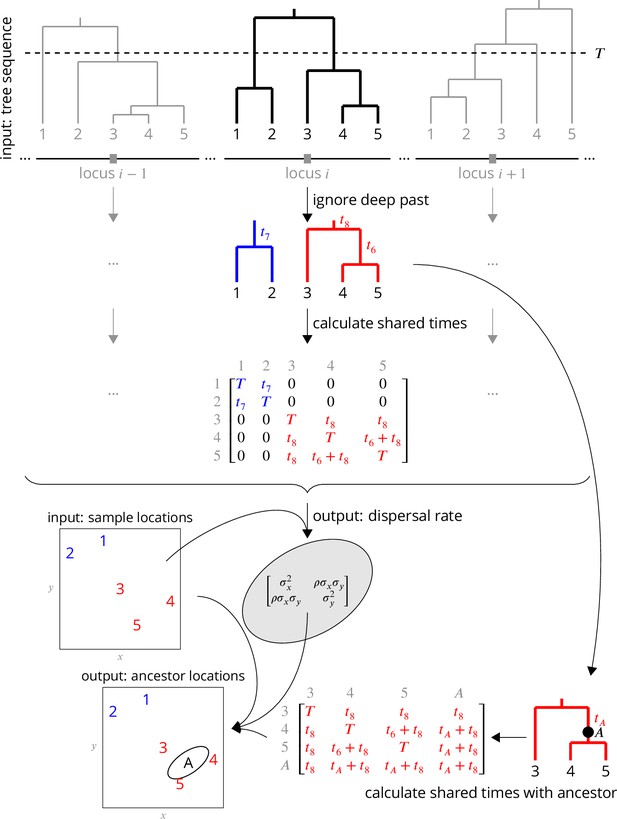
Conceptual overview of the approach.
From a sequence of trees covering the full genome, we downsample to trees at approximately unlinked loci. To avoid the influence of strongly non-Brownian dynamics at deeper times (e.g., glacial refugia, boundaries), we ignore times deeper than , which divides each tree into multiple subtrees (here, blue and red subtrees at locus ). From these subtrees, we extract the shared times of each pair of lineages back to the root. In practice (but not shown here), we use multiple samples of the tree at a given locus, for importance sampling, and also extract the coalescence times for importance sample weights. Under Brownian motion, the shared times describe the covariance we expect to see in the locations of our samples, and so using the times and locations we can find the maximum likelihood dispersal rate (a 2 × 2 covariance matrix). While we can estimate a dispersal rate at each locus, a strength of our approach is that we combine information across many loci, by multiplying likelihoods, to estimate a single genome-wide dispersal rate. Finally, we locate a genetic ancestor at a particular locus (a point on a tree, here ) by first calculating the time this ancestor shares with each of the samples in its subtree, and then using the shared times and dispersal rate to calculate the probability distribution of the ancestor’s location conditioned on the sample locations. In practice (but not shown here), we calculate the location of the ancestor of a given sample at a given time across many loci, combining information across loci into a distribution of genome-wide ancestry across space.
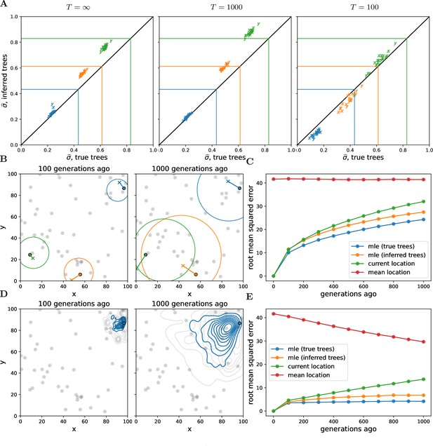
Simulations.
(A) Accuracy of genome-wide dispersal rates. Maximum composite likelihood estimates of dispersal rate (in ‘x’ and ‘y’ dimensions) using the true trees vs. Relate-inferred trees for three different time cutoffs, . Colours indicate the simulated dispersal rates, which are given by the corresponding lines. (B) Locating genetic ancestors at a particular locus. 95% confidence ellipses for the locations of genetic ancestors for three samples at a single locus (using the true trees and the simulated dispersal rate). The ‘o’s are the sample locations and the ‘x’s are the true ancestral locations. (C) Accuracy of locating genetic ancestors at individual loci. Root mean squared errors between the true locations of ancestors and the mean location of the samples (red), the current locations of the samples (green), and the maximum likelihood estimates from the inferred (orange) and true (blue) trees. (D) Locating genetic ancestors at many loci. Contour plots of the most likely (using the true trees; blue) and the true (grey) locations of genetic ancestors at every 100th locus for a given sample. (E) Accuracy of mean genetic ancestor locations. Root mean squared errors between the true mean location of genetic ancestors and the mean location of the samples (red), the current locations of the samples (green), and the mean maximum likelihood estimates from the inferred (orange) and true (blue) trees. To reduce computation time we only attempt to locate the first 10 samples. In all panels, there are 10 replicate simulations for each combination of time cutoff and dispersal rate. We sample 50 diploid individuals at random and use every 100th locus, with 1000 importance samples at each. Panels B–E have no time cutoff, , and were simulated with a dispersal rate given by green lines in panel A. In panels C and E, the inferred tree ancestor location estimates use the inferred tree dispersal estimates.
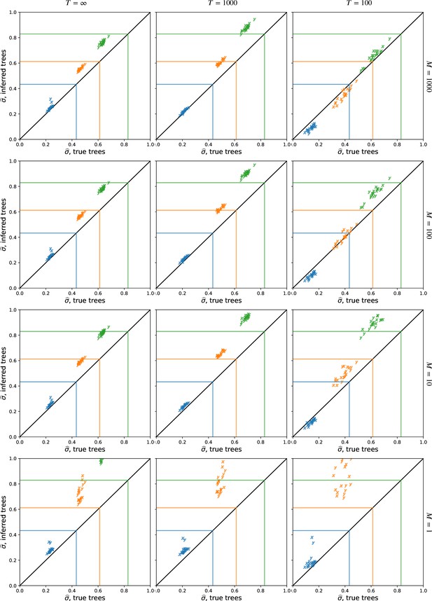
The effect of importance sampling on dispersal estimates.
Importance sampling more trees, , at each locus brings the dispersal estimate from the inferred trees closer to the dispersal estimate from the true trees and lowers the variance in dispersal estimates across replicates. See Figure 2 for more information, where (top row).
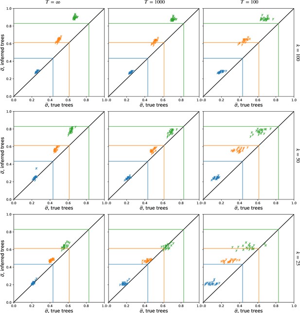
The effect of sample size on dispersal estimates.
Using more samples, , tends to increase the dispersal estimate from both true and inferred trees and reduce the variation in estimates across replicates at smaller cutoff times. See Figure 2 for more information, where , and we sample every 100th locus. To isolate the effect of larger trees (rather than more trees), here we use the first sampled loci. To speed up calculations, here we use importance samples at each locus.
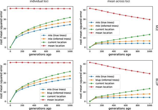
Comparing maximum likelihood estimate (MLE) and best linear unbiased predictor (BLUP) ancestor locations.
The top row shows error in the MLE ancestor locations (orange), as in Figure 2, while the bottom row shows the error in the BLUP ancestor locations (orange). The methods are very comparable, though the BLUP method may do slightly worse at estimating the mean ancestor location at deep times.
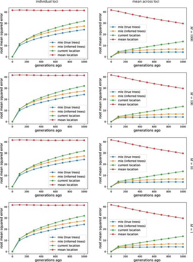
The effect of importance sampling on ancestor location estimates.
See Figure 2 for more information, where (top row).
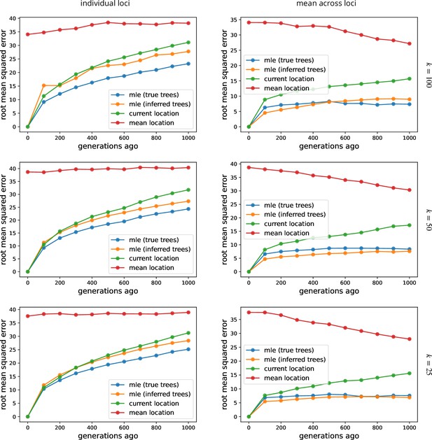
The effect of sample size on ancestor location estimates.
See Figure 2 for more information, where , , and we sample every 100th locus. To isolate the effect of larger trees (rather than more trees), here we use the first sampled loci. To speed up calculations, here we use importance samples at each locus.
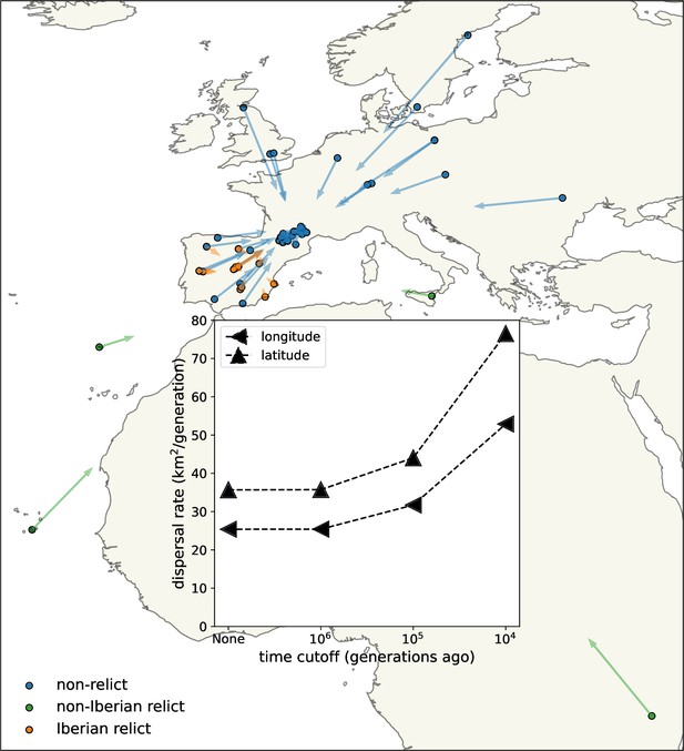
Dispersal rates (inset) and major trends in geographic ancestries.
Vectors start at sample locations (circles) and point to the mean location of ancestors across 878 loci 104 generations ago. Samples coloured by genomic principle component group (Wlodzimierz et al., 2023).
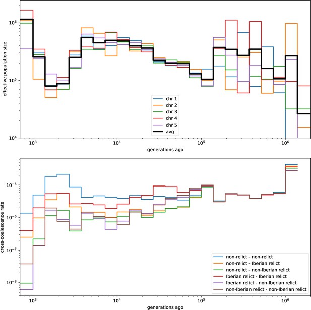
Relate-inferred effective population sizes and cross-coalescent rates.
Effective population sizes for each chromosome (top) and cross-coalescence rates for each pair of principle component groups (bottom) inferred with Relate. Compare with Figure 4a in 1001 Genomes Consortium, 2016 and Figures 5 and 6 in Durvasula et al., 2017.
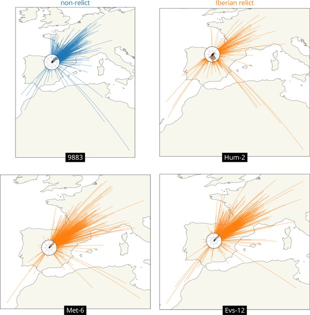
Visualizing the geographic sources of ancestry.
Great circles connecting sample and ancestor locations at 878 loci 104 generations ago. Polar histograms (windroses) show the distribution of direction in ancestral locations from the sample. Non-relicts in blue, Iberian relicts in orange.

Visualizing the movement of geographic ancestries over time.
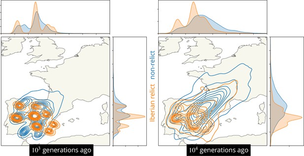
Ancestor locations at 878 loci (circles) and kernel density estimates (contours). Non-relicts in blue, non-Iberian relcits in green.


