Research Article

Physics of Living Systems

Learning to predict target location with turbulent odor plumes

Department of Physics, University of Genova, Italy
Institut de Physique de Nice, Université Côte d’Azur, Centre National de la Recherche Scientifique, France
National Institute of Nuclear Physics, Italy
MalGa, Department of Civil, Chemical and Environmental Engineering, University of Genoa, Italy
MaLGa, Department of computer science, bioengineering, robotics and systems engineering, University of Genova, Italy

Aug 12, 2022

https://doi.org/10.7554/eLife.72196

7 figures, 1 table and 1 additional file

Figures

Figure 1 with 1 supplement

Download asset Open asset

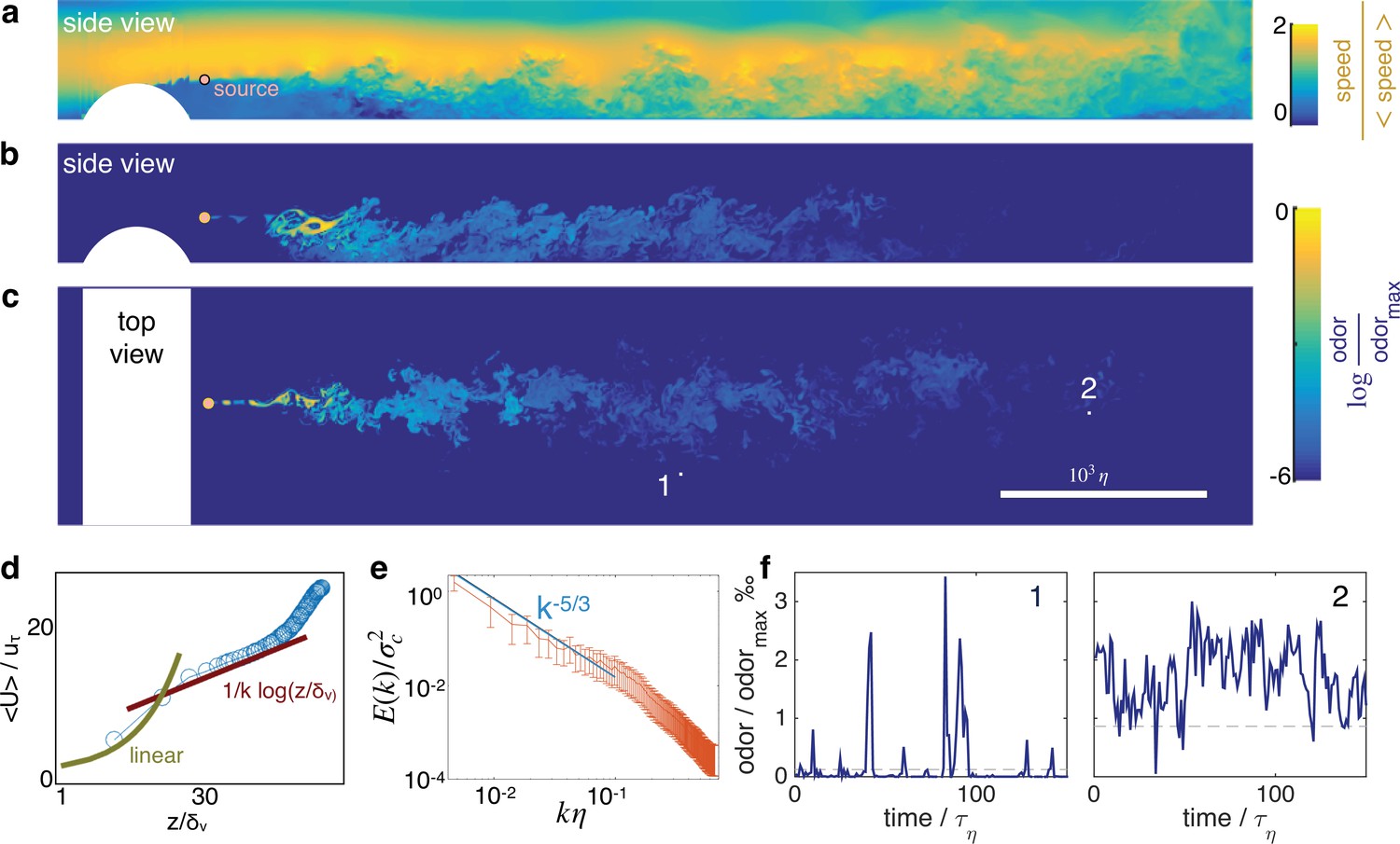
Turbulent odor cues are patchy and intermittent.

Snapshot of streamwise velocity (a) in a vertical plain at mid channel; odor snapshot side view at mid channel (b) and top view at source height (c). White regions mark the cylindrical obstacle. Snapshots are obtained from direct numerical simulations of the Navier-Stokes equations and the equation for odor transport (see Materials and Methods and parameters summarized in Table 1). (d) The mean velocity profile follows the well known log law when $z_{3}^{+}$ = $z_{3} / δ_{ν}$ > 30, where $δ_{ν} = ν / u_{τ}$ where $u_{τ}$ is the friction velocity. (e) Two dimensional spectra of odor fluctuations $E (k) = \frac{d}{d k} (\int_{| k_{x y} | < k} | \hat{c} (k_{x y}) |^{2} d^{2} k)$ normalized with the scalar variance $σ_{c}^{2}$ ; $\hat{c} (k_{x, y})$ is the 2D Fourier transform of the scalar concentration at source height; the integral of the spectra is the scalar variance. Wavenumbers are nondimensionalized with the inverse Kolmogorov scale $η^{- 1}$ . Error bars show standard deviation calculated over N = 420 points. (f) Typical time courses of the odor cues at locations labeled with 1 and 2 in c, visualizing noise and sparsity, particularly at location 1.

Figure 1—video 1

Download asset

posterframe for video — Direct numerical simulations of the turbulent flow in a channel of length L, width W and height H evolving in time.

Figure 2 with 6 supplements

Download asset Open asset

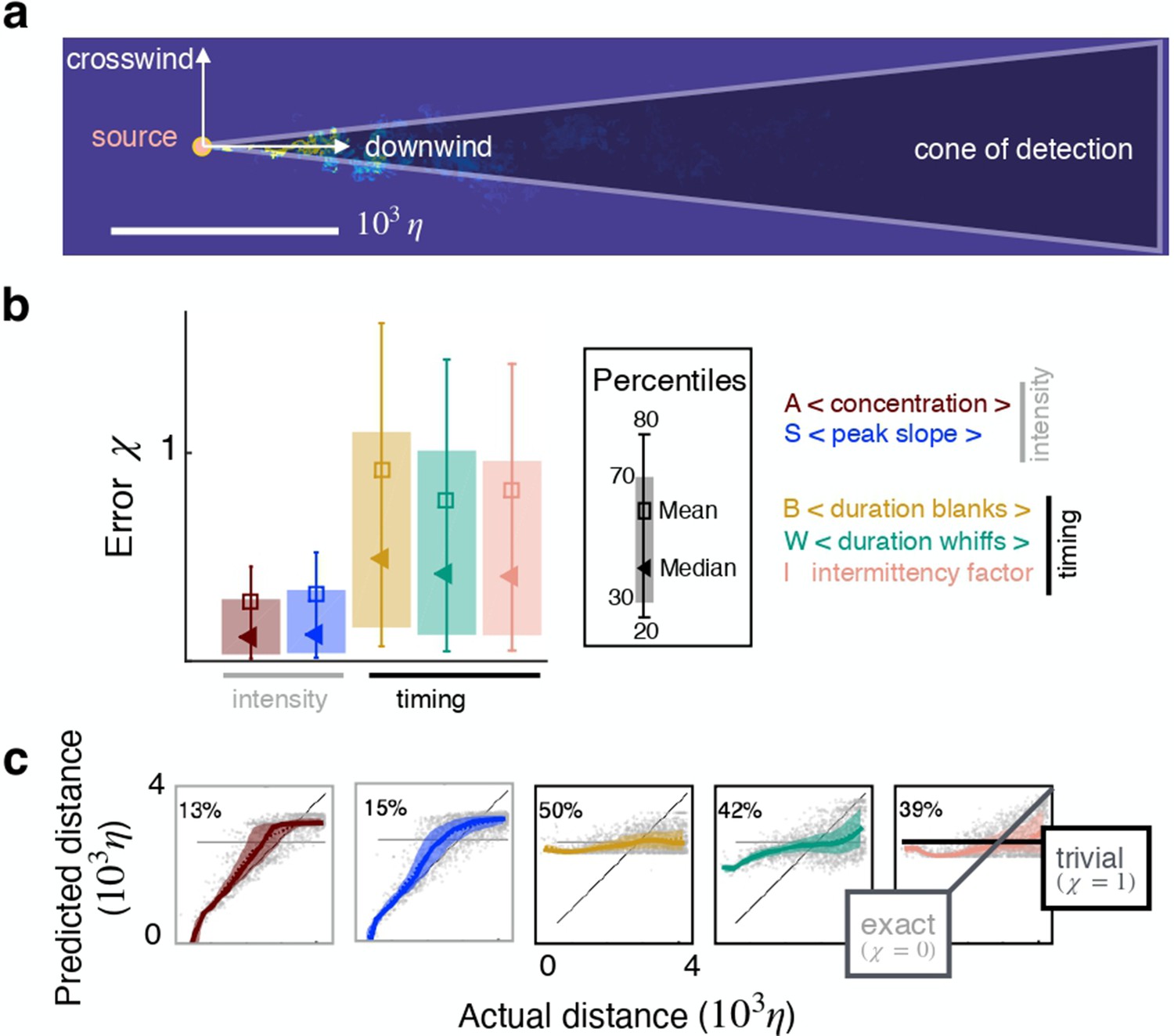
Individual features enable inference in two dimensions.

(a) Sketch of the geometry. (b) Test error $χ$ for inference using individual features as input. (c) Predicted vs actual distance for inference. Prediction for representative test points (grey circles); 30–70th percentile (patch, same color code as in (b)); trivial prediction $f (x) =< y >_{test}$ (solid horizontal line, corresponds to $χ = 1$ ); exact prediction (bisector, corresponds to $χ = 0$ ); dispersion away from the bisector visualizes the prediction error. Results are obtained with a supervised learning algorithm based on regularized empirical risk minimization (Materials and methods). Each input datum x_i is one individual scalar feature computed from the time course of odor concentration measured at location $z_{i}$ at 100 evenly spaced time points with sampling frequency $ω = 1 / τ_{η}$ , where $τ_{η}$ is Kolmogorov time. The training/test set are composed of $N = 5000$ and $N_{t} = 13500$ data points, respectively.

Figure 2—figure supplement 1

Download asset Open asset

Fixed vs adaptive threshold.

Test error using an adaptive threshold (left column) vs a fixed threshold (right column) for different simulations described in the main text. Adaptive thresholds are defined as a fraction of the local average concentration, $< c >_{local}$ , computed over the memory $M / ω$ . Fixed thresholds are defined as a fraction of the global maximum concentration c₀. Results are robust with respect to the choice of adaptive threshold, whereas they vary considerably with the choice of fixed thresholds. Large fixed thresholds (marked with yellow squares) prevent odor detection in dilute regions that is far from the source or from the substrate.

Figure 2—figure supplement 2

Download asset Open asset

Linear least square algorithm.

Prediction error for a least squares algorithm assuming the target function is a linear function of the input (no regularization). Performance is poor regardless of the input features and the dataset (dataset A to E are defined as for Figure 5).

Figure 2—figure supplement 3

Download asset Open asset

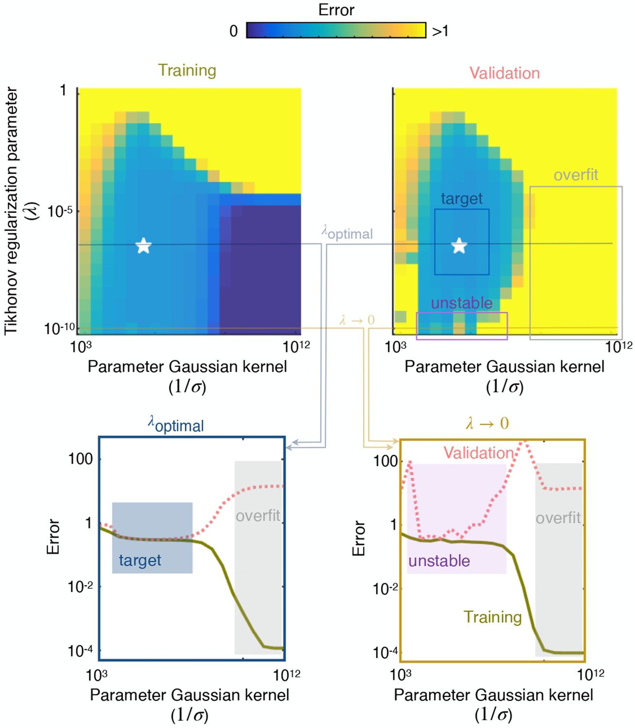
Visualisation of a typical cross validation procedure.

Visualisation of a typical cross validation procedure, exemplifying the need for regularization for this problem. Left and right color plots show the error on the training set (left) and test set (right) as a function of the two hyperparameters $λ$ (Tikhonov regularization parameter) and $σ$ (width of the Gaussian kernel), see Materials and methods for more details. Bottom: test and training errors for $λ \to 0$ as a function of $1 / σ$ . For large values of $1 / σ$ , the solution overfits the data and for small values of $1 / σ$ , the solution does not overfit but is unstable. Top: test and training errors for $σ \to 0$ as a function of $λ$ . For large values of $1 / σ$ , the solution overfits the data and for small values of $1 / σ$ , the solution does not overfit but is unstable.

Figure 2—figure supplement 4

Download asset Open asset

Test error at source height, for prediction in the crosswind direction.

Symbols as in Figure 2.

Figure 2—figure supplement 5

Download asset Open asset

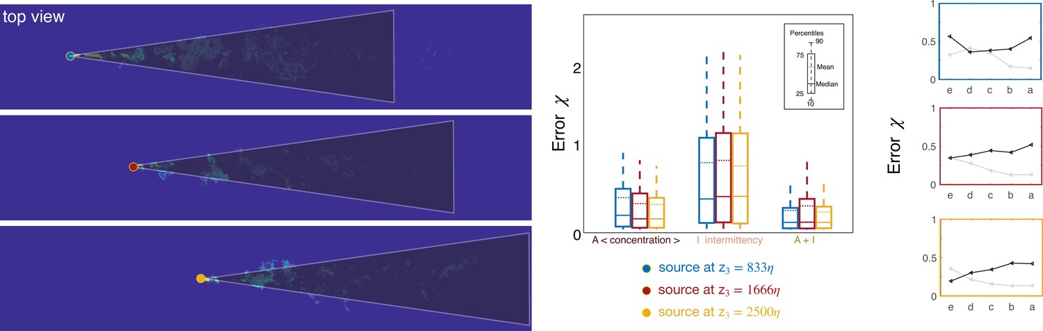
Results for three source locations.

Results vary little when the source is moved downstream of its original position. Left: sketch of the three source positions and conical domain used for training. Center: test error at source height for two individual features (average and intermittency) as well as their combination, as indicated on x-axis. Right: test error for two individual features (average, grey line and intermittency, black line) at five different heights marked with a to e as in Figure 5.

Figure 2—figure supplement 6

Download asset Open asset

Results of training with odor emanating from one source and testing over odor fields emanating from the other two.

The algorithm is robust to source location. Left: performance of the pair average concentration and intermittency. Center: performance of the individual feature average concentration. Right: performance of individual feature intermittency. Boxes extend from the $25^{t h}$ to the $75^{t h}$ percentile; dashed line: median. Green: training and test are performed over the same dataset; blue: test is performed over the simulation with odor source closest to the obstacle; dark red: test is over the dataset obtained with the middle source; yellow: test is over the dataset with the source furthest downstream. Training dataset are indicated on the $x$ -axis.

Figure 3 with 2 supplements

Download asset Open asset

The sampling strategy affects performance but not ranking.

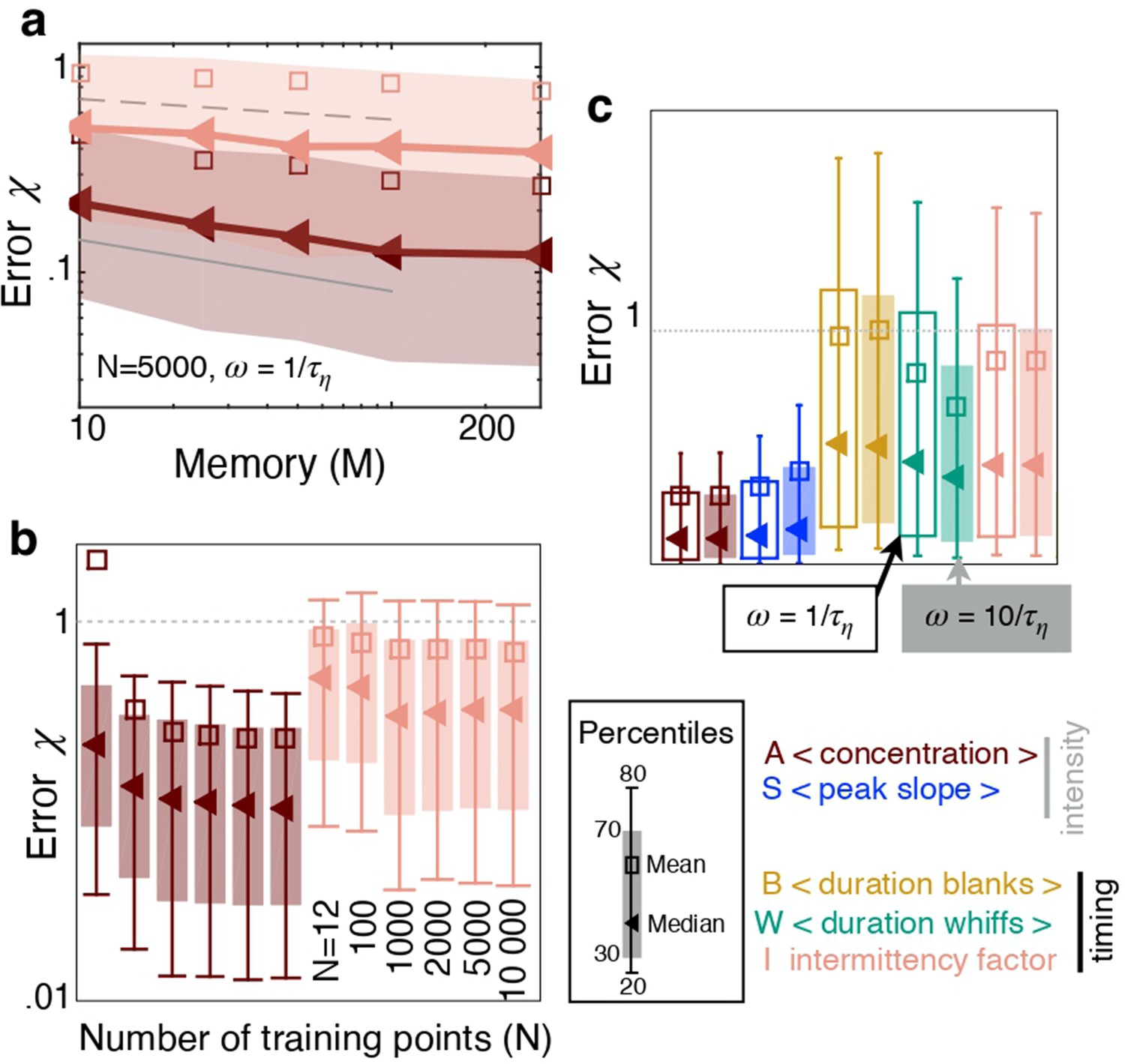
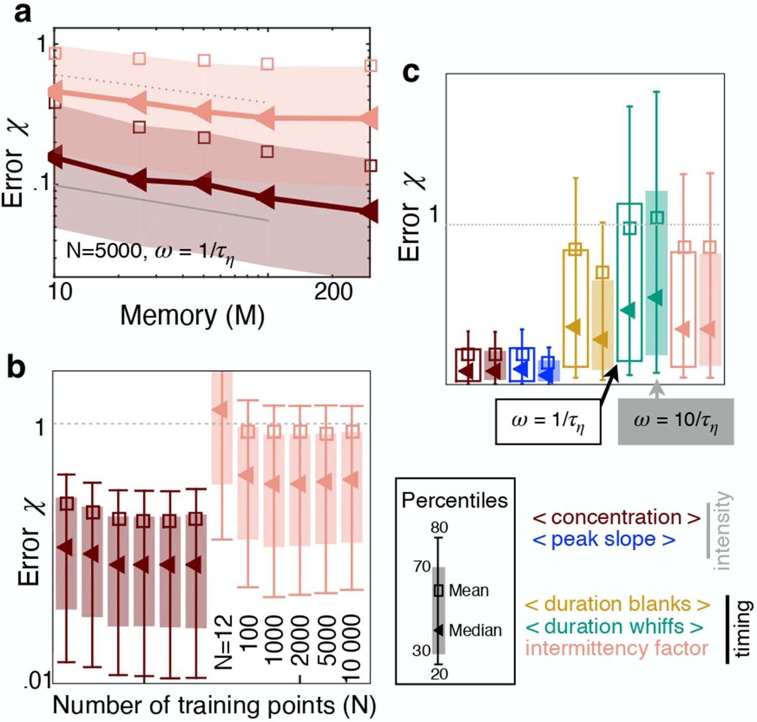
(a) Error $χ$ as a function of memory in units of Kolmogorov times $τ_{η}$ ; memory is defined as the duration of the time series of odor concentration $c_{i} = (c (z_{i}, t_{i}), \dots, c (z_{i}, t_{i + M}))$ used to compute the five features $x_{i}^{1}, \dots, x_{i}^{5}$ , i.e. memory $= t_{i + M} - t_{i} = M / ω$ . Red and pink: Performance using $x_{i} = x_{i}^{1}$ (average concentration) and $x_{i} = x_{i}^{5}$ (intermittency factor). The number of training points and the frequency of sampling are fixed, $N = 5000$ and $ω = 1 / τ_{η}$ . Dotted, dashed and solid grey lines are power laws with exponents $- 1 / 5$ , $- 1 / 10$ and $- 1 / 4$ respectively to guide the eye. (b) Error as a function of number of points in the training set $N$ , with $N_{t} = 13500$ points in the test set, memory $= 100 τ_{η}$ and $ω = 1 / τ_{η}$ . Color code as in (a). (c) Performance using the five individual features as input with $N = 5000$ , $N_{t} = 13500$ , memory $= 100 τ_{η}$ sampling odor at frequency $ω = 1 / τ_{η}$ (empty bars) and $ω = 10 / τ_{η}$ (filled bars). Key shows color coding.

Figure 3—figure supplement 1

Download asset Open asset

Prediction error as a function of the number of points in the training set for individual features and pairs of features.

Based on this analysis we chose N=5000.

Figure 3—figure supplement 2

Download asset Open asset

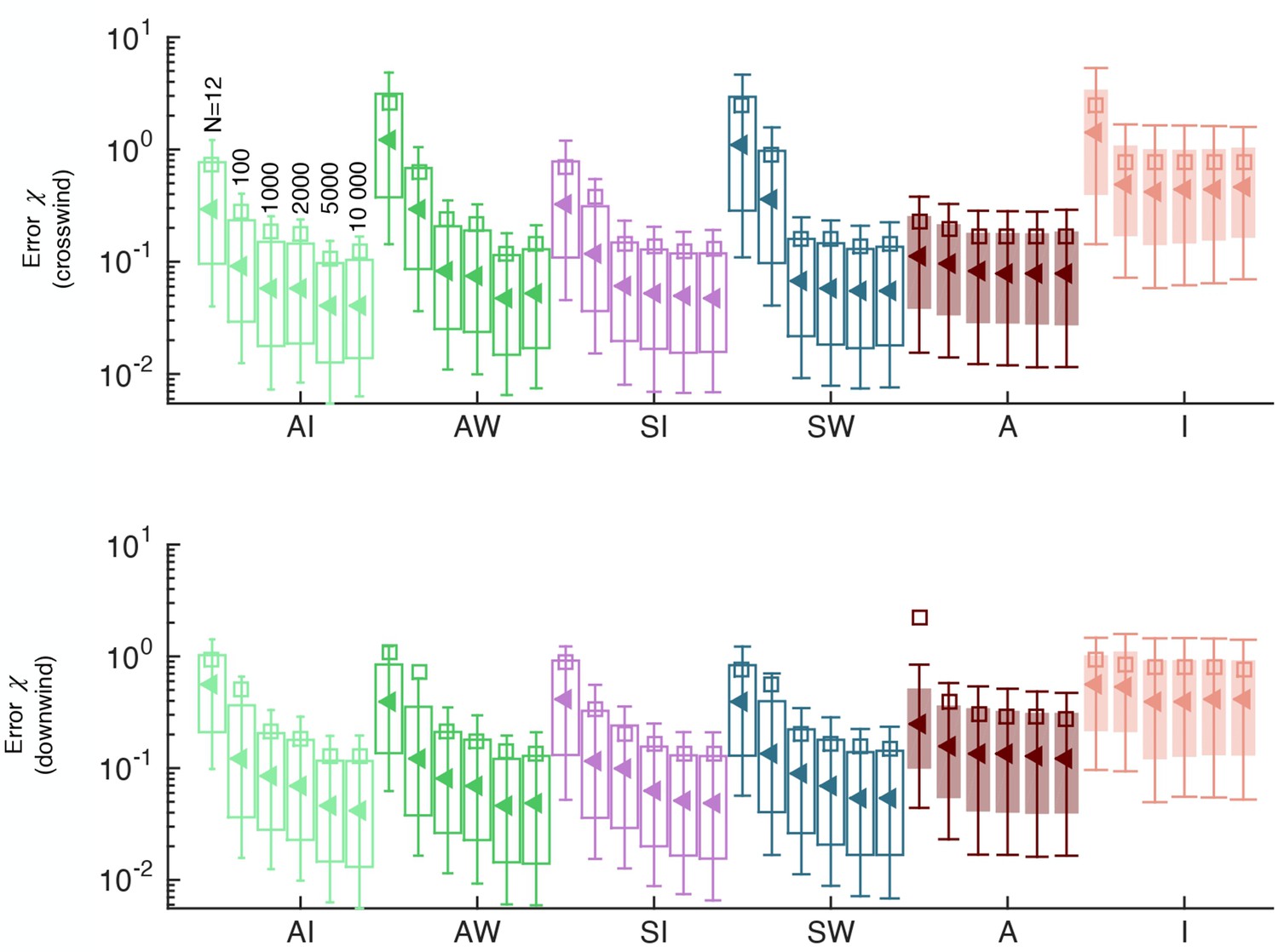
Effect of memory, sampling frequency and number of points in the training set, for prediction in the crosswind direction.

Symbols as in Figure 3.

Figure 4 with 1 supplement

Download asset Open asset

Pairing one timing feature and one intensity feature considerably improves performance.

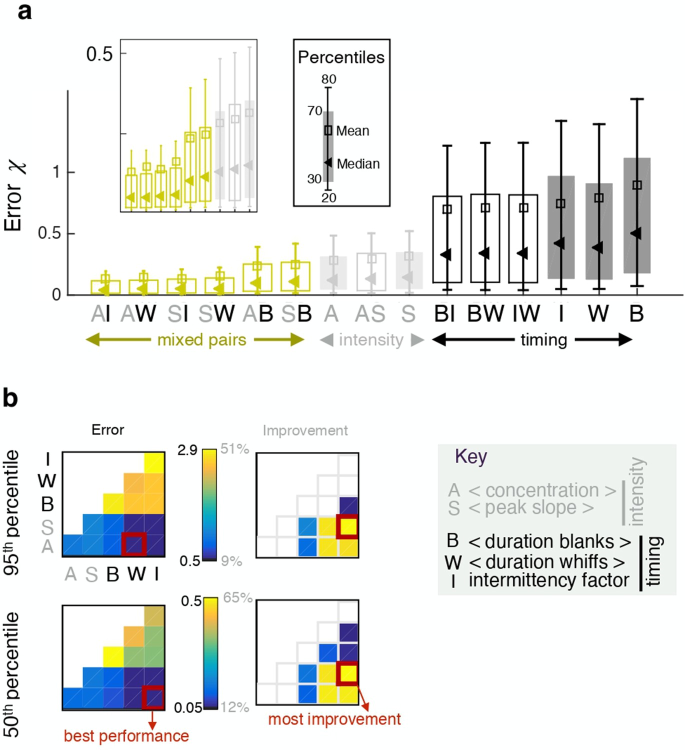
(a) Error $χ$ obtained with individual features (full bars) and pairs of features (empty bars). Grey and black indicate pairings of two intensity features and two timing features respectively; green indicates mixed pairs of one timing and one intensity feature. (b) Performance (left) and relative improvement over the best of the two paired features (right). Results for the median (bottom) and the 95th percentile (top). Within each table plot, rows from bottom to top and columns from left to right are labeled by the 5 individual features: A (average, $x^{1}$ ), S (slope $x^{2}$ ), B (blanks $x^{3}$ ), W (whiffs $x^{4}$ ), I (intermittency $x^{5}$ ). Results with individual features are shown on the diagonal; results pairing feature $i$ and feature $j$ are shown at position $(i, j)$ . Mixed pairs provide both the best performance and the largest improvement over individual features.

Figure 4—figure supplement 1

Download asset Open asset

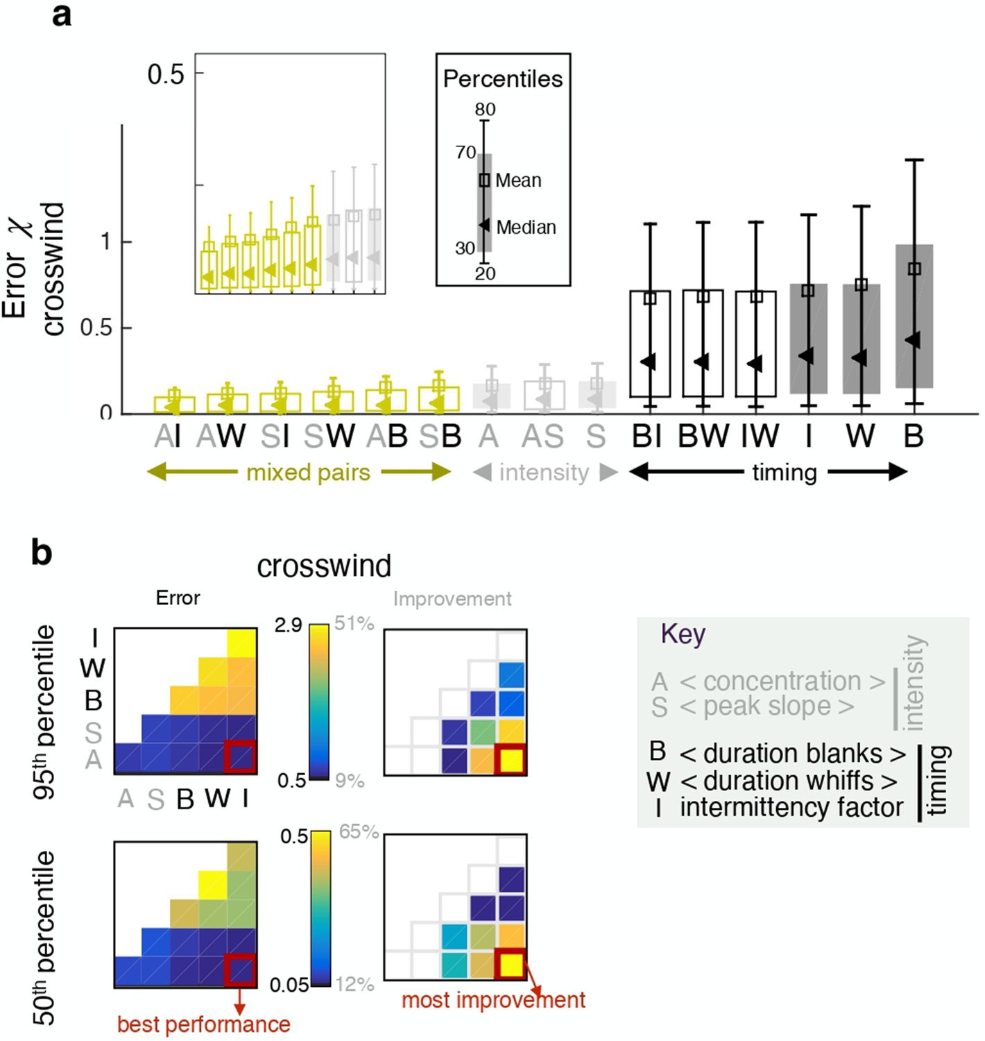
Effect of pairing two individual features, for prediction in the crosswind direction.

Symbols as in Figure 4.

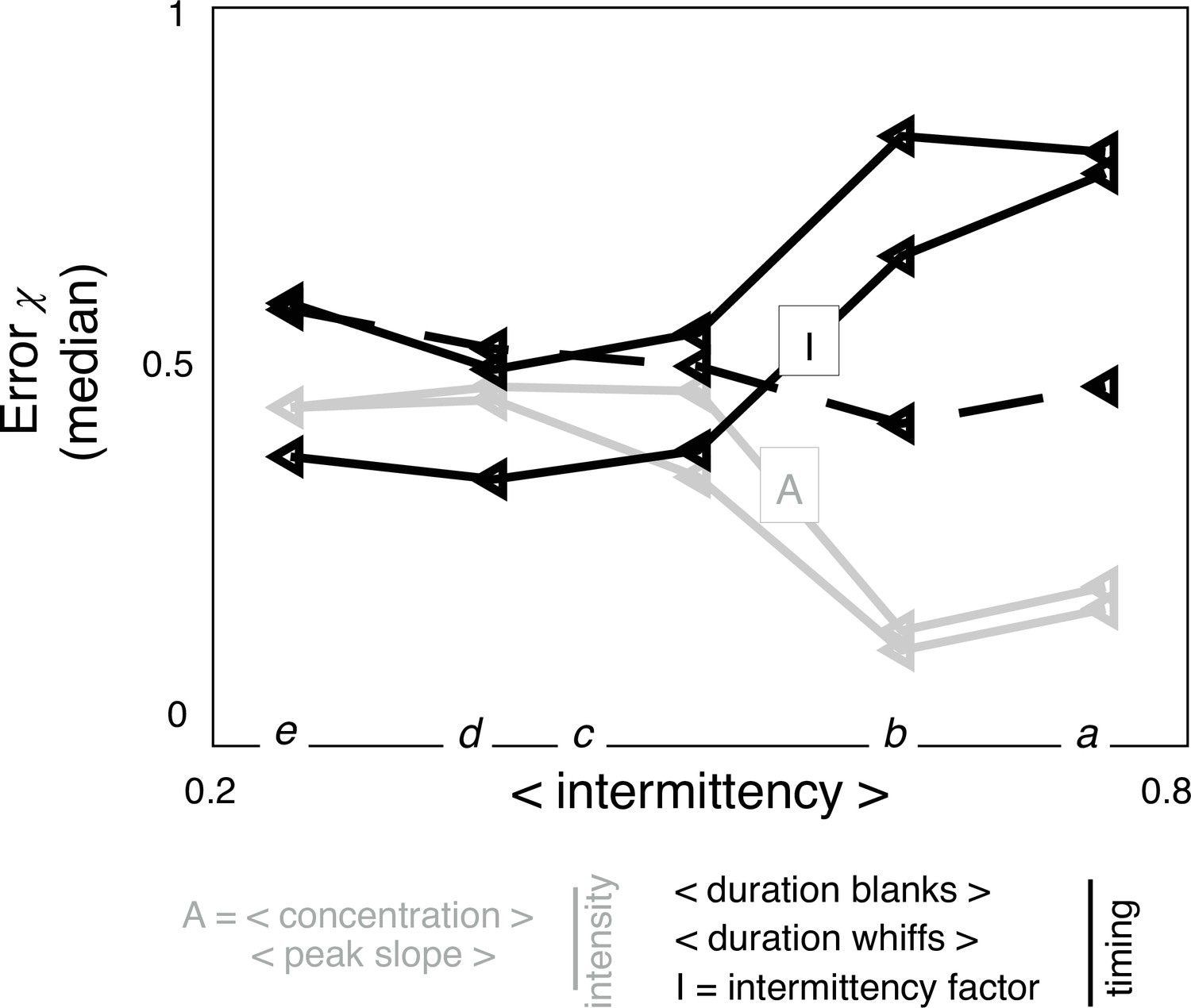
Figure 5 with 3 supplements

Download asset Open asset

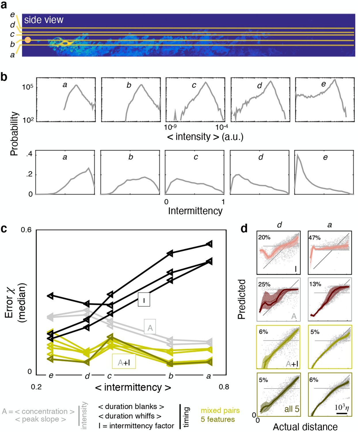
Ranking shifts with height from the ground.

(a) Datasets a to e correspond to data obtained at heights $z / H = 25 %$ , 37.5%, 50%, 55% and 65% respectively. (b) Distribution of intensities (top) and intermittency factors (bottom) over the training set from a to e (left to right). Moving away from the boundary, the odor becomes less intense and more sparse. (c) Median performance as a function of average intermittency factor of the training set for individual intensity (grey) and timing (black) features, mixed pairs of one intensity and one timing feature (green) and all five features together (dark green). (d) Predicted vs actual distance, to visualize a representative subset of the results in (c), scale bar $10^{3} η$ . Ranking depends sensibly on height: intensity features outperform timing features near the substrate, where there is more odor and it is more continuous; timing features outperform intensity features further from the substrate where there is less odor and it is more sparse; mixed pairs perform best across all conditions; combining five features provides little to no improvement over mixed pairs.

Figure 5—figure supplement 1

Download asset Open asset

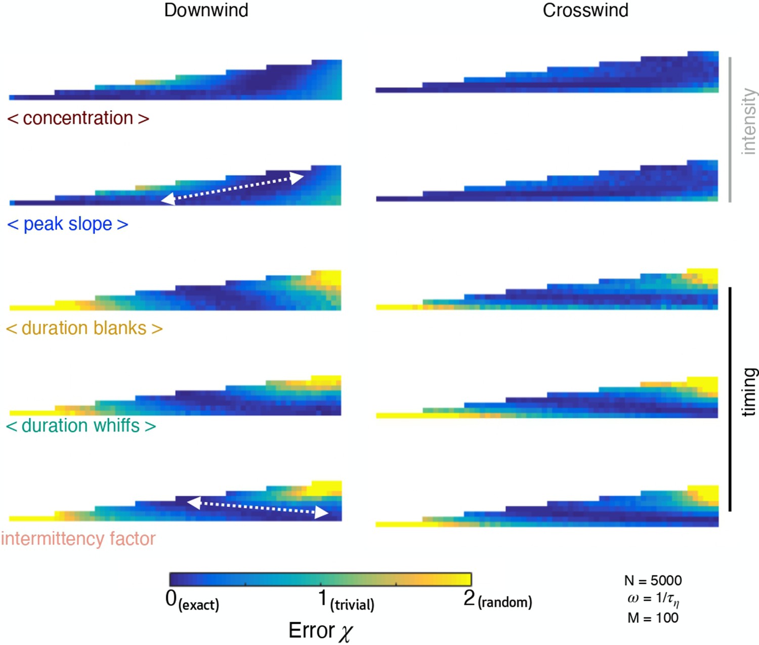
Test error mapped in space.

Test error mapped in space for a kernel ridge regression algorithm that takes individual observables in input and predicts distance in the downwind (left) and crosswind (right) direction for simulation b. The test error is color coded from 0 (blue) to 2 (yellow) corresponding to the limits of perfect prediction and random prediction.

Figure 5—figure supplement 2

Download asset Open asset

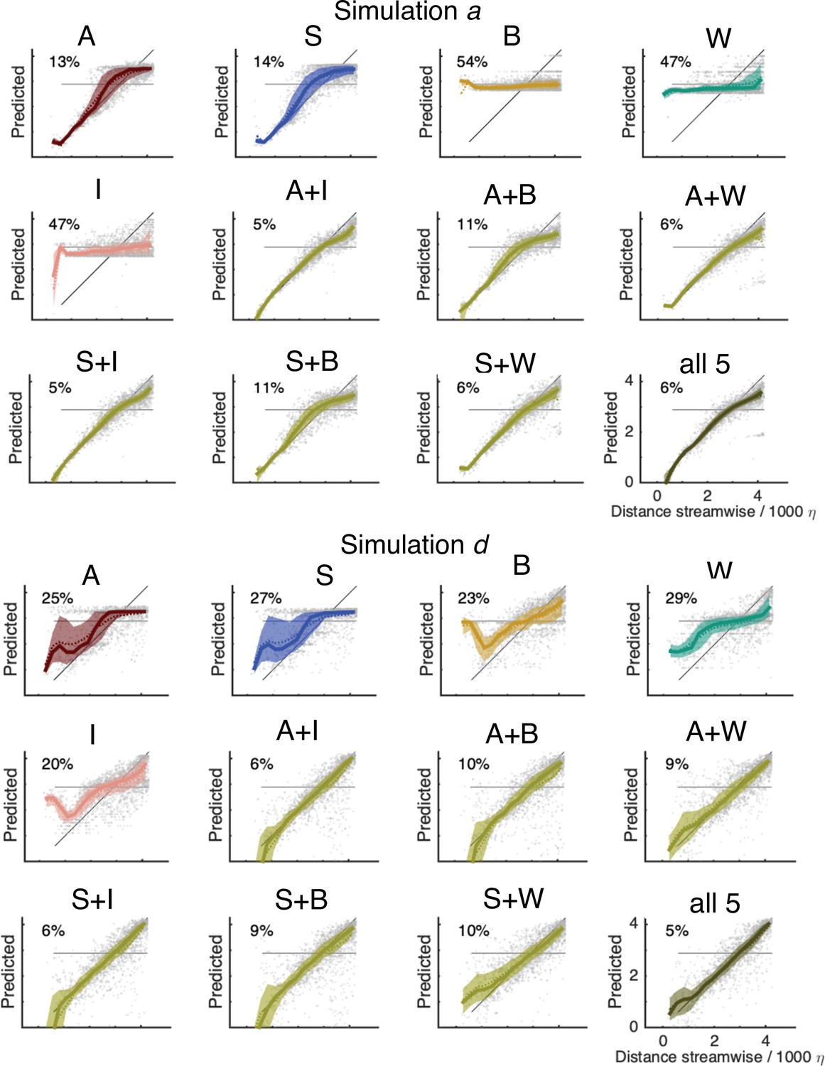
Predicted distance vs actual distance for simulation a (top) and (d) (bottom); symbols as in Figure 5d.

The bisector corresponds to a perfect prediction; departure from the bisector visualizes the error.

Figure 5—figure supplement 3

Download asset Open asset

Estimated predicted power of individual features.

Estimated test error of individual features at different heights using the theoretical framework Equations 5–10 outlined in the text and Materials and methods, using an estimate of the likelihood obtained empirically from our data (not shown). Symbols as in Figure 5c (black / grey represent timing /intensity features; dashed lines: whiffs).

Figure 6

Download asset Open asset

Ranking depends on distance from the source.

(a) At source height, the dataset is split in proximal (distance <2330η) and distal (distance >2330η). (b) Distributions of average odor intensity (left) and intermittency factor (right) over the training set; closer to the source, the odor is more intense and more sparse. (c) Distribution of test error for the proximal (left) and distal (right) problem showing intensity features (grey) outperform timing features (black) at close range, but not in the distal problem where differences in the error distribution are limited to the tails (see insets). Mixed pairs of features (green) outperform individual features either marginally (left) or considerably (right). (d) Percentiles of the error distribution in (c) for the proximal (left) and distal (right) problems confirming the picture emerged from (c).

Author response image 1

Download asset Open asset

Estimated test error of individual features at different heights using the theoretical framework Equation (1)-(5) outlined in the text with the empirical likelihood estimated from data (not shown).

Symbols as in Figure 5c of the manuscript (black / grey represent timing /intensity features; dashed lines: whiffs).

Tables

Table 1

Parameters of the simulation.

Length $L$ , width $W$ , height $H$ of the computational domain; horizontal speed along the centerline $U$ ; mean horizontal speed $U_{b} = ⟨ u ⟩$ ; kinematic viscosity $ν$ ; diffusivity $κ_{c}$ ; Kolmogorov length scale $η = {(ν^{3} / ϵ)}^{1 / 4}$ where $ϵ$ is the energy dissipation rate; mean size of gridcell $Δ x$ ; Kolmogorov timescale $τ_{η} = η^{2} / ν$ ; energy dissipation rate $ϵ = ν / 2 ⟨ {(\partial u_{i} / \partial x_{j} + \partial u_{j} / \partial x_{i})}^{2} ⟩$ ; Taylor microscale $λ = \sqrt{⟨ u^{2} ⟩ / ⟨ {(\partial u / \partial x)}^{2} ⟩}$ ; wall lengthscale $y^{+} = ν / u_{τ}$ where the friction velocity is $u_{τ} = \sqrt{τ / ρ}$ and the wall stress is $τ = {ρ ν d u / d z |}_{z = 0}$ ; Reynolds number $R e = U (H / 2) / ν$ based on the centerline speed $U$ and half height; Reynolds number $R e_{λ} = U λ / ν$ based on the centerline speed and the Taylor microscale $λ$ ; Schmidt number (Sc = $ν / κ_{c}$ = Pe/Re); magnitude of velocity fluctuations $u^{'}$ relative to the centerline speed; large eddy turnover time $T = H / 2 u^{'}$ . First row reports results in non dimensional units; second and third rows correspond to dimensional parameters in air and water assuming the velocity of the centerline is 50 cm/s in air and 12 cm/s in water.

	$L$	$W$	$H$	$U$	$U_{b}$	$ν$	$κ_{c}$	$η$	$Δ x$
	40	8	4	32	23	1/250	1/250	0.006	0.025
air	9.50 m	1.90 m	0.96 m	50 cm/s	36 cm/s	1.510^-5 m²/s	1.510^-5 m²/s	0.15 cm	0.6 cm
water	2.66 m	0.53 m	0.27 m	12 cm/s	8.6 cm/s	10^-6 m²/s	10^-6 m²/s	0.04 cm	0.2 cm
	$τ_{η}$	ε	λ	y⁺	Re	Re_λ	Sc	$u^{'} / U$	$T$
	0.01	39	0.17	0.0035	16000	1360	1	11%	$64 τ_{η}$
air	0.15 s	6.3e-4 m²/s³	4 cm	0.09 cm
water	0.18 s	3e-5 m²/s³	1 cm	0.02 cm

Additional files

MDAR checklist: https://cdn.elifesciences.org/articles/72196/elife-72196-mdarchecklist1-v1.docx
Download elife-72196-mdarchecklist1-v1.docx

Download links

A two-part list of links to download the article, or parts of the article, in various formats.

Downloads (link to download the article as PDF)

Open citations (links to open the citations from this article in various online reference manager services)

Mendeley

Cite this article (links to download the citations from this article in formats compatible with various reference manager tools)

Nicola Rigolli
Nicodemo Magnoli
Lorenzo Rosasco
Agnese Seminara

(2022)

Learning to predict target location with turbulent odor plumes

eLife 11:e72196.

https://doi.org/10.7554/eLife.72196

Share this article

Cite this article

Turbulent odor cues are patchy and intermittent.

Direct numerical simulations of the turbulent flow in a channel of length L, width W and height H evolving in time.

Individual features enable inference in two dimensions.

Fixed vs adaptive threshold.

Linear least square algorithm.

Visualisation of a typical cross validation procedure.

Test error at source height, for prediction in the crosswind direction.

Results for three source locations.

Results of training with odor emanating from one source and testing over odor fields emanating from the other two.

The sampling strategy affects performance but not ranking.

Prediction error as a function of the number of points in the training set for individual features and pairs of features.

Effect of memory, sampling frequency and number of points in the training set, for prediction in the crosswind direction.

Pairing one timing feature and one intensity feature considerably improves performance.

Effect of pairing two individual features, for prediction in the crosswind direction.

Ranking shifts with height from the ground.

Test error mapped in space.

Predicted distance vs actual distance for simulation a (top) and (d) (bottom); symbols as in Figure 5d.

Estimated predicted power of individual features.

Ranking depends on distance from the source.

Estimated test error of individual features at different heights using the theoretical framework Equation (1)-(5) outlined in the text with the empirical likelihood estimated from data (not shown).

Parameters of the simulation.

MDAR checklist

Downloads (link to download the article as PDF)

Open citations (links to open the citations from this article in various online reference manager services)

Cite this article (links to download the citations from this article in formats compatible with various reference manager tools)