Figures and data in A unified framework for measuring selection on cellular lineages and traits

Figures
Tables
Additional files

8 figures, 4 tables and 1 additional file

Figures

Figure 1

Download asset Open asset

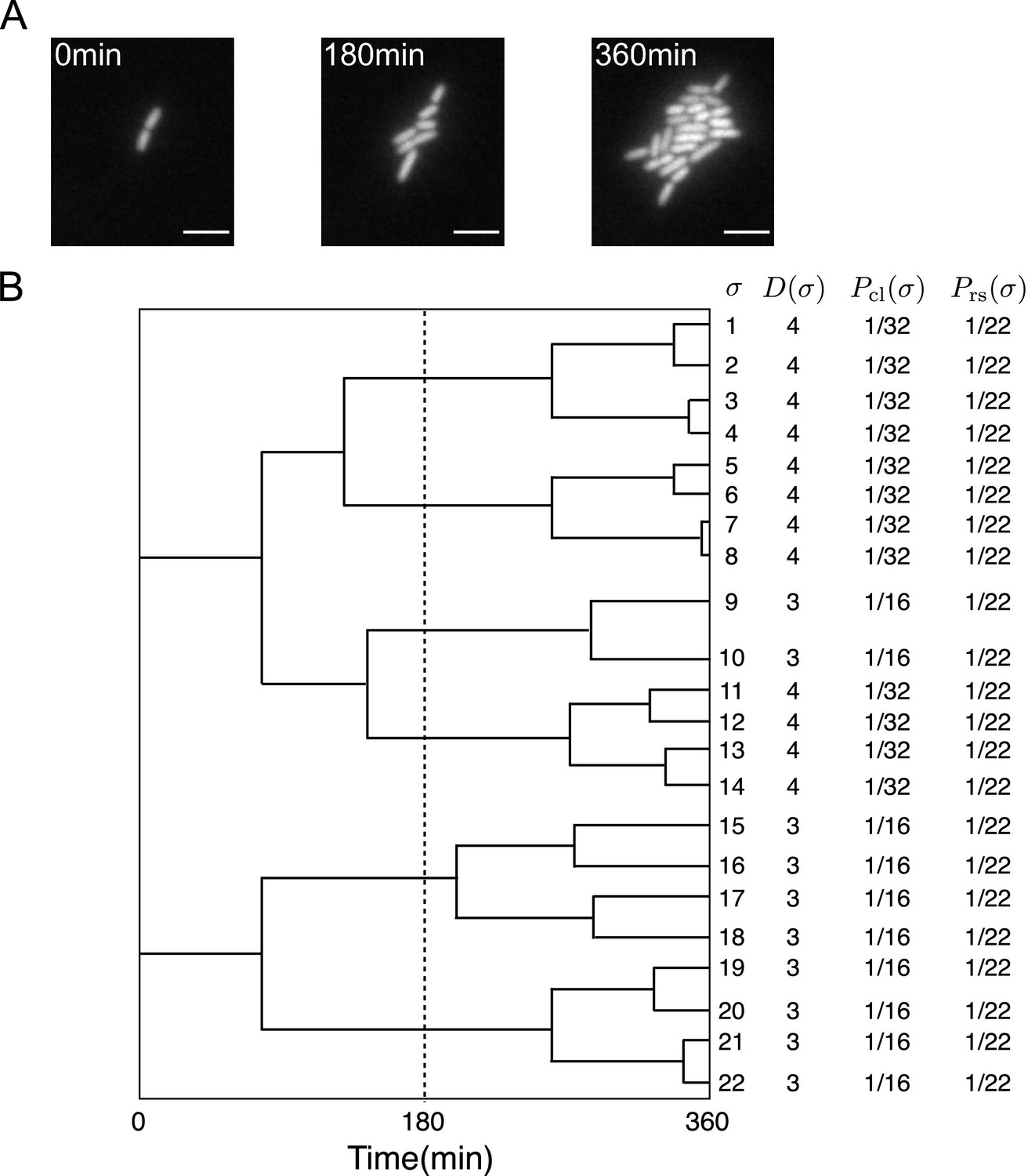
Representative single-cell lineage trees.

(A) Time-lapse images of a growing microcolony of *Escherichia coli* expressing green fluorescent protein (GFP) from plasmids. Scale bars, 5 μm. (B) Cellular lineage trees for the microcolony in A. Bifurcations in the trees represent cell divisions. $σ$ denotes cell lineage labels. $D (σ)$ shows the number of cell divisions in each lineage. $P_{cl} (σ)$ and $P_{rs} (σ)$ are chronological and retrospective probabilities defined in the main text.

Figure 2

Download asset Open asset

Conceptual illustration of the relationships between fitness landscapes, trait distributions, and selection strength.

(A) Non-uniform fitness landscape and broad trait distribution. The gray distribution represents a chronological distribution of lineage trait $x$ ; the cyan distribution represents a retrospective distribution of lineage trait $x$ ; and the black dashed line represents a fitness landscape. Due to the non-uniform fitness landscape and the broad chronological distribution, there is trait fitness heterogeneity for selection to act on. The retrospective distribution therefore shifts significantly from the chronological distribution, and the selection strength is large ( $S [X] > 0$ ). (B) Non-uniform fitness landscape and narrow trait distribution. Due to the lack of trait heterogeneity, there is little fitness heterogeneity for selection to act on. The retrospective distribution shifts only slightly from the chronological distribution, and the selection strength is small ( $S [X] \approx 0$ ). (C) Uniform fitness landscape. When the fitness landscape is constant ( $= τ Λ$ ) across the lineage trait state $x$ , there can be no trait fitness heterogeneity regardless of whether the trait distribution itself is narrow or broad. The selection strength is therefore zero ( $S [X] = 0$ ).

Figure 3

Download asset Open asset

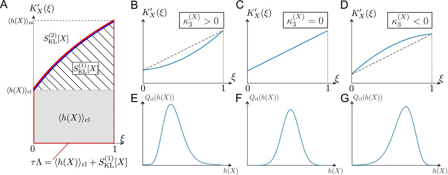
Relationships among chronological distributions’ shape and selection strength measures.

(A) Graphical representation of various fitness and selection strength measures by $K_{X}^{'} (ξ)$ -plot. Blue curve represents $K_{X}^{'} (ξ)$ . The area between the horizontal axis and $K_{X}^{'} (ξ)$ in the interval $0 \leq ξ \leq 1$ outlined in red corresponds to population growth $τ Λ$ . The gray and hatched regions correspond to ${⟨ h (X) ⟩}_{cl}$ and $S_{KL}^{(1)} [X]$ , respectively. The area between $K_{X}^{'} (ξ)$ and $y = {⟨ h (X) ⟩}_{rs}$ corresponds to $S_{KL}^{(2)} [X]$ . (**B-D**) Representative shapes of $K_{X}^{'} (ξ)$ depending on $κ_{3}^{(X)}$ . Assuming that the contributions from fourth or higher-order cumulants are negligible, $K_{X}^{'} (ξ)$ becomes convex downward when $κ_{3}^{(X)} > 0$ (B); a straight line when $κ_{3}^{(X)} = 0$ (C); and convex upward when $κ_{3}^{(X)} < 0$ (D). (**E-G**) Relationships between third-order fitness cumulant and skewness of chronological distribution $Q_{cl} (h)$ .

Figure 4 with 1 supplement

Download asset Open asset

Population growth rate response to cell removal perturbation.

(A) Scheme of random cell removal. Here, we consider the situation where cells were removed probabilistically after each cell division. Red crosses represent cell removal positions in the tree. The lineages after cell removal points disappear from the tree. Consequently, the number of cells at the end time point decreases. (B) Generation time distributions used in the simulation. We assumed that cellular generation time follows gamma distributions in the simulation. We set the shape parameter to either 1 ( $g_{1} (x)$ ), 2 ( $g_{2} (x)$ ), or 5 ( $g_{3} (x)$ ). (**C-E**) Population growth rate changes by cell removal perturbation. Gray points show the relative changes in population growth rate $Δ Λ / Λ := (Λ (ϵ) - Λ (0)) / Λ (0)$ . Cell removal probability was set to $1 - 2^{- ϵ}$ in each condition of perturbation strength $ϵ$ . Broken red lines represent the theoretical prediction $Δ Λ / Λ \approx - \frac{{⟨ \tilde{h} (D) ⟩}_{rs}}{τ Λ} ϵ = - (1 + \frac{S_{KL}^{(2)} [D]}{τ Λ}) ϵ$ . The lines of $Δ Λ / Λ = - ϵ$ (blue) and $- \frac{{⟨ \tilde{h} (D) ⟩}_{cl}}{τ Λ} ϵ$ (green) are shown for reference. The generation time distributions used in the simulation are $g_{1} (x)$ for C, $g_{2} (x)$ for D, and $g_{3} (x)$ for E.

Figure 4—figure supplement 1

Download asset Open asset

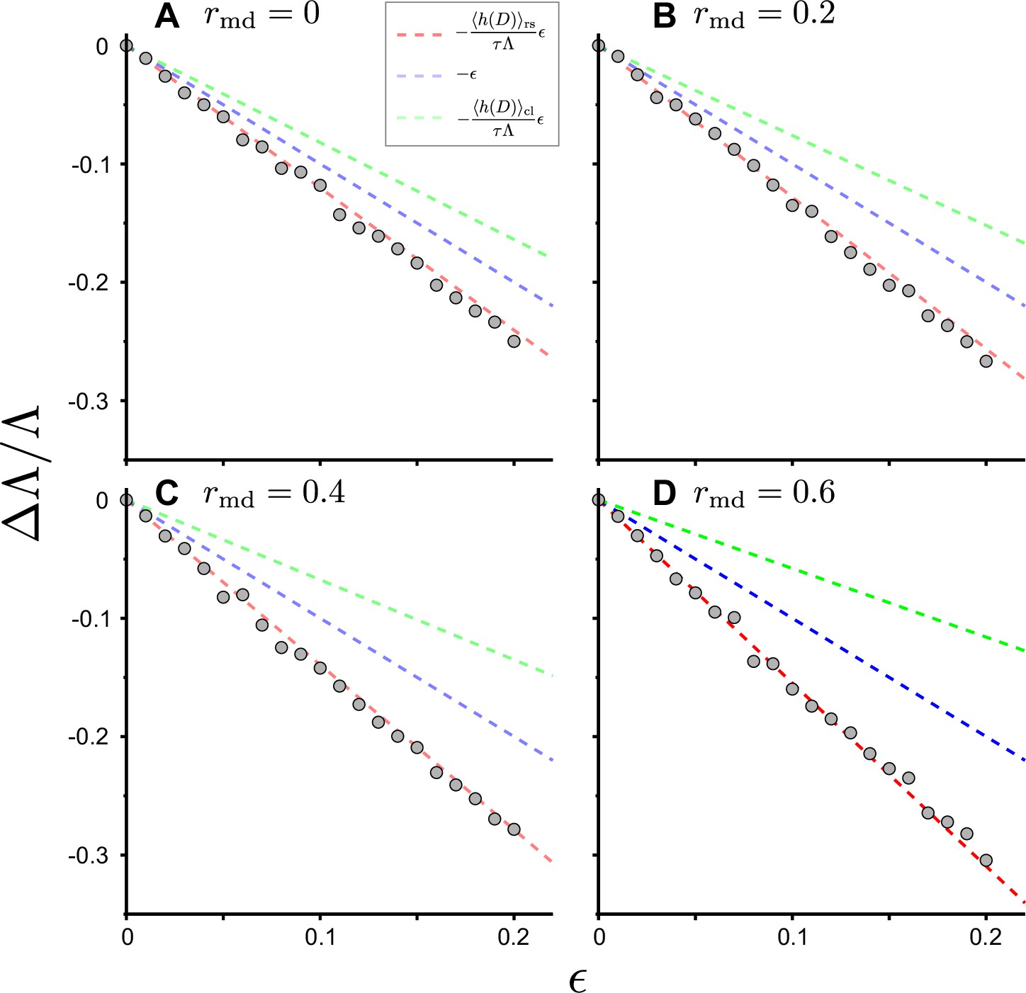
Response of population growth rate to cell removal perturbation with positive mother-daughter correlations of generation time.

We conducted the simulations of cell population growth with positive mother-daughter correlations (Gray points). We considered the generation time distribution that follows a gamma distribution with shape parameter 2 ( $g_{2} (x)$ in Figure 4B). We generated correlated generation time of individual cells based on the mother cell’s value with the algorithm in Materials and methods. We randomly removed the individual cells from the population with the probability $1 - 2^{- ϵ}$ after each cell division. The broken red lines represent the theoretical prediction of the changes $Δ Λ / Λ = - \frac{{⟨ \tilde{h} (D) ⟩}_{rs}}{τ Λ} ϵ$ . The lines of $Δ Λ / Λ = - ϵ$ (blue) and $Δ Λ / Λ = - \frac{{⟨ \tilde{h} (D) ⟩}_{cl}}{τ Λ} ϵ$ (green) were also shown for reference. (A) The result with no mother-daughter correlation of generation time ( $r_{md} = 0$ ). (B) $r_{md} = 0.2$ . (C) $r_{md} = 0.4$ . (D) $r_{md} = 0.6$ .

Figure 5 with 2 supplements

Download asset Open asset

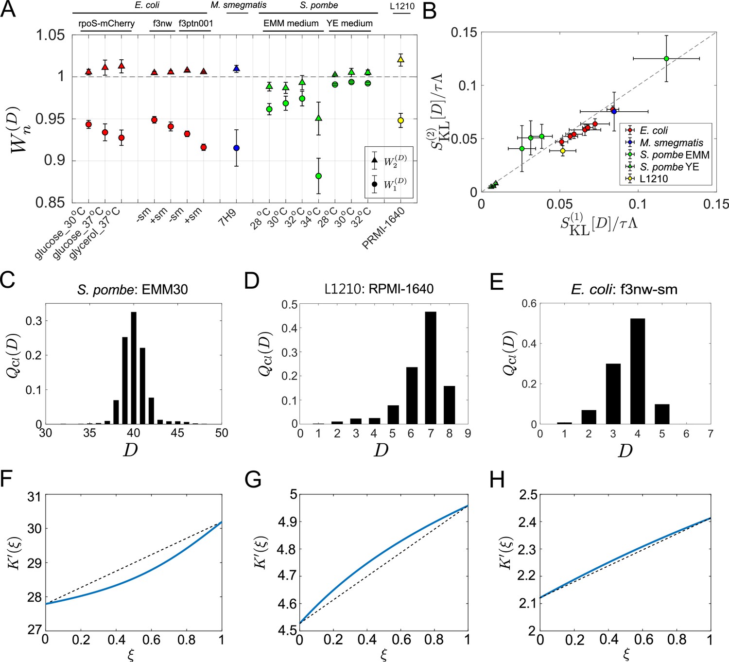
Application of cell lineage statistics to experimental data.

(A) Contributions of the cumulants of a fitness landscape to population growth. $W_{1}^{(D)}$ and $W_{2}^{(D)}$ were evaluated for the experimental cell lineage data from *E. coli* (red), *M. smegmatis* (blue), *S. pombe* (green), and L1210 mouse leukemia cells (yellow). The *E. coli* rpoS-mcherry data were newly obtained in this study (see Materials and methods). The other data were taken from literature: *E. coli* f3nw and f3ptn001 from Nozoe et al., 2017; *M. smegmatis* from Wakamoto et al., 2013; *S. pombe* from Nakaoka and Wakamoto, 2017; and L1210 from Seita et al., 2021. Circles and triangles represent $W_{1}^{(D)}$ and $W_{2}^{(D)}$ , respectively. Error bars represent the two standard deviation ranges estimated by resampling the cellular lineages (see Materials and methods). (B) Relationship between $S_{KL}^{(1)} [D] / τ Λ$ and $S_{KL}^{(2)} [D] / τ Λ$ . Colors correspond to the cellular species as in A. The *S. pombe* data were further categorized into two groups: Circles for the EMM conditions; and triangles for the YE conditions. (**C-E**) Representative chronological distributions of division count, $Q_{cl} (D)$ . (**F-H**) Graphical representation of $K_{D}^{'} (ξ)$ . F for *S. pombe* EMM30; G for L1210 RMPI-1640; and H for *E. coli* f3nw-sm.

Figure 5—figure supplement 1

Download asset Open asset

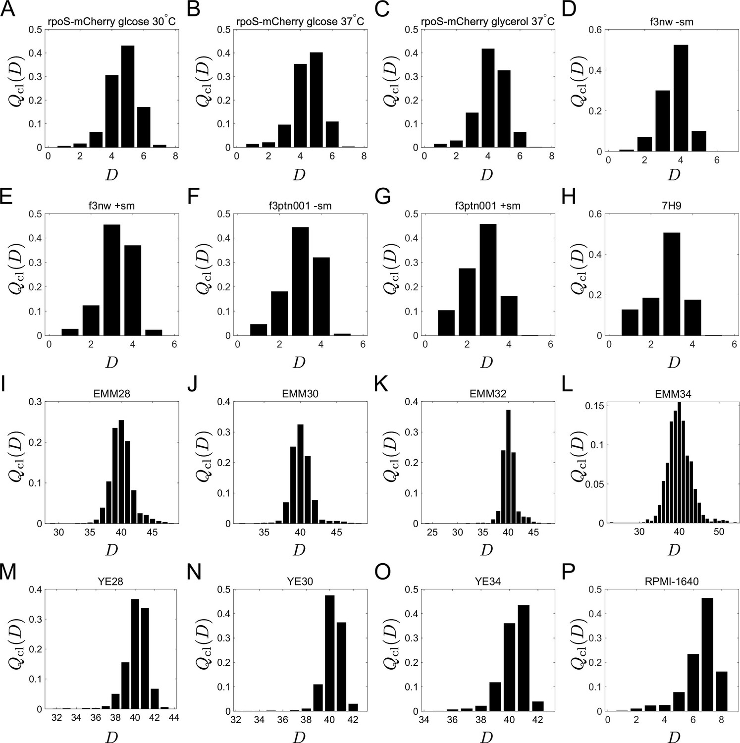
Chronological distributions of division count, $Q_{cl} (D)$ .

(**A-G**) *E. coli*. (H). *M. smegmatis*. (**I-O**) *S. pombe*. P. L1210 mouse leukemia cells.

Figure 5—figure supplement 2

Download asset Open asset

Graphical representation of $K_{D}^{'} (ξ)$ .

A-G. *E. coli*. H. *M. smegmatis*. I-O. *S. pombe*. P. L1210 mouse leukemia cells.

Figure 6

Download asset Open asset

Strong selection in the E.coli population regrowing from a late stationary phase.

(A) Time-lapse images. Cellular regrowing dynamics from early and late stationary phases were observed by time-lapse microscopy. Cells were enclosed in the microchambers etched on coverslips. The top three images show representative images of the cells from an early stationary phase. The bottom three images show the cells from a late stationary phase. Scale bar, 5 μm. (B) Population dynamics. The number of cells at each time point normalized by the initial cell number ( $N (t) / N (0)$ ) was plotted against time $t$ was 307 for the early stationary sample and 295 for the late stationary sample. (**C, D**) Representative cellular lineage trees in the regrowing kineics from the early stationary phase (C) and the late stationary phase (D). The trees correspond to the time-lapse images in A. (E) Cumulative contributions of the cumulants of the fitness landscape $h (D)$ to population growth. Error bars represent the two standard deviation ranges estimated by resampling the cellular lineages (see Materials and methods). (F) Chronological distributions of division count $Q_{cl} (D)$ . (G) Relationships between $S_{KL}^{(1)} [D]$ and $S_{KL}^{(2)} [D]$ . The blue and black points show the results for the early stationary phase sample and the late stationary phase sample, respectively. Gray points represent the results for the cell populations growing at approximately constant growth rates shown in Figure 5B.

Figure 7 with 1 supplement

Download asset Open asset

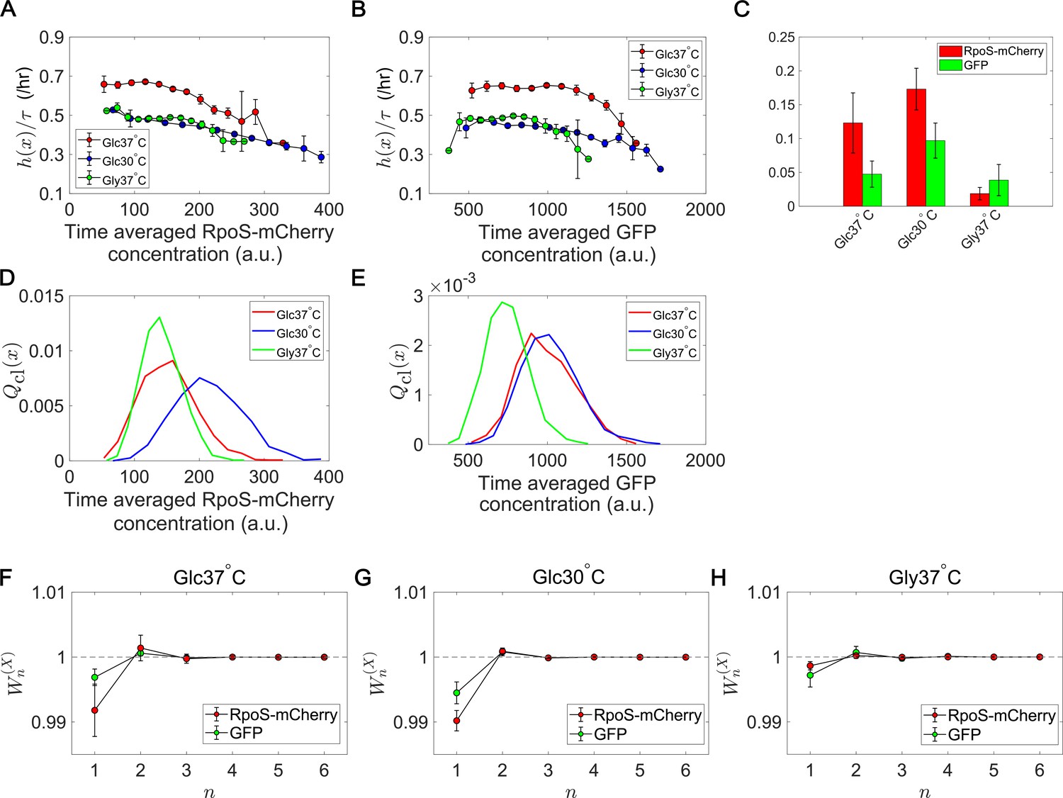
Fitness landscapes and selection strength for RpoS expression levels.

(A) Fitness landscapes for the time-averaged concentration (mean fluorescent intensity) for RpoS-mCherry. The time-averaged mean fluorescent intensity of RpoS-mCherry was adoped as a lineage trait $X$ and changes in fitness were plotted against the trait values $x$ . Fitness landscapes were scaled by the lineage length (observation duration) $τ$ . Error bars represent the two standard deviation ranges estimated by resampling the cellular lineages. (B) Fitness landscapes for the time-averaged concentration for GFP. The time-averaged mean fluorescent intensity of GFP was adoped as a lineage trait $X$ and changes in fitness were plotted against the trait values $x$ . (C) Relative selection strength for the time-averaged concentrations of RpoS-mCherry (red) and GFP (green). (**D, E**) Chronological distributions $Q_{cl} (x)$ for the time-averaged concentrations of RpoS-mCherry (D) and GFP (E). (**F-H**) Cumulative contributions of fitness cumulants to population growth, $W_{n}^{(X)}$ , assuming that $X$ is either time-averaged concentration of RpoS-mCherry (red) or time-averaged concentration of GFP (green). Error bars represent the two standard deviation ranges estimated by resampling the cellular lineages. Panel F is for the Glucose-37°C condition; Panel G for the Glucose-30°C condition; and Panel H for the Glycerol-37°C condition.

Figure 7—figure supplement 1

Download asset Open asset

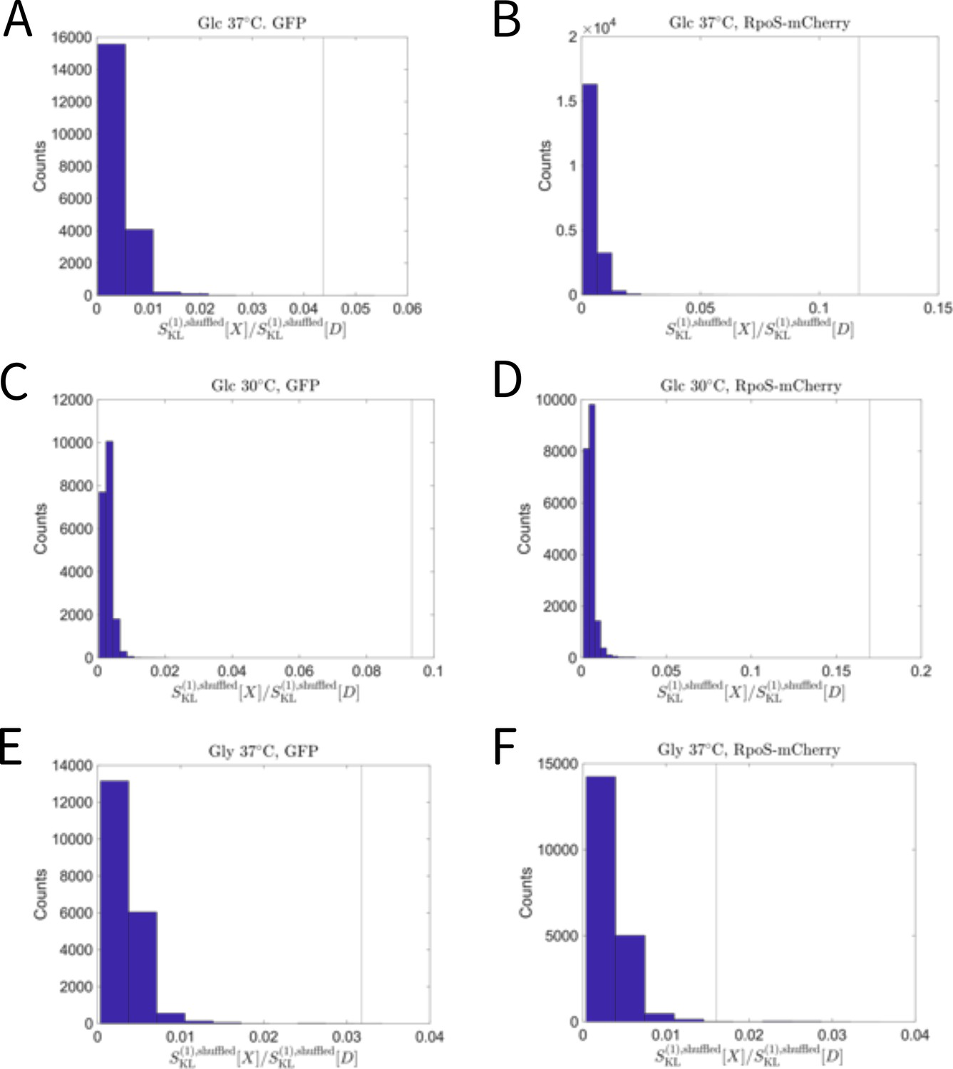
The relative selection strength values for time-averaged RpoS-mCherry and GFP fluorescence intensity compared with the randomized data.

The blue histograms show the distributions of the relative selection strength values calculated from the lineage data in which the correspondences between division counts and trait values are shuffled. The vertical lines indicate the relative selection strength values for the experimental data. A. GFP under the Glucose-37°C condition. B. RpoS-mCherry under the Glucose-37°C condition. C. GFP under the Glucose-30°C condition. D. RpoS-mCherry under the Glucose-30°C condition. E. GFP under the Glycerol-37°C condition. F. RpoS-mCherry under the Glycerol-37°C condition.

Appendix 1—figure 1

Download asset Open asset

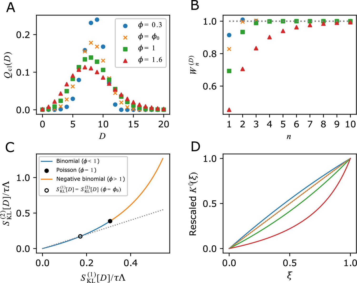
Analytical calculations of $K_{D} (ξ)$ and related relations given specific form of division count distributions.

(A) Chronological division count distributions. $ϕ = 0.3$ and $ϕ = ϕ_{0} (= 0.5857 \dots)$ are binomial, $ϕ = 1$ is Poisson and $ϕ = 1.6$ is negative binomial. $\bar{D} = 20 (1 - ϕ_{0})$ is fixed. (B) Cumulative contributions of fitness cumulants. Parameter values are given in panel A legend. (C) The relation between two selection strength measures. Binomial (blue curve), Poisson (closed black circle) and negative binomial (orange curve) are indicated on the single curve plotted using Equations 37 and 38 within the range of $0 < ϕ < 2$ . The point where $S_{KL}^{(1)} [D] = S_{KL}^{(2)} [D]$ ( $ϕ = ϕ_{0}$ ) is indicated by the open black circle. The grey dotted line corresponds to $S_{KL}^{(1)} [D] = S_{KL}^{(2)} [D]$ . (D) Convexity of $K_{D}^{'} (ξ)$ . Y-axis shows a rescaling of $K_{D}^{'} (ξ)$ according to $(K_{D}^{'} (ξ) - K_{D}^{'} (0)) / (K_{D}^{'} (1) - K_{D}^{'} (0))$ . The same values of $ϕ$ as in A are used; $ϕ = 0.3$ (blue), $ϕ = ϕ_{0}$ (orange), $ϕ = 1$ (green) and $ϕ = 1.6$ (red). The grey dotted line indicates the case that $K_{D}^{'} (ξ)$ is a linear function of $ξ$

Tables

Table 1

Relationships between $K_{X} (ξ)$ and quantities in cellular lineage statistics.

	Quantities in lineage statistics	Symbol	Correspondence to $K_{X} (ξ)$
Fitness	Population growth	$τ Λ$	$K_{X} (1)$
	Chronological mean fitness	${⟨ h (X) ⟩}_{cl}$	$K_{X}^{'} (0)$
	Retrospective mean fitness	${⟨ h (X) ⟩}_{rs}$	$K_{X}^{'} (1)$
	Chronological fitness variance	$Var {[h (X)]}_{cl}$	$K_{X}^{''} (0)$
	Retrospective fitness variance	$Var {[h (X)]}_{rs}$	$K_{X}^{''} (1)$
Selection strength	Jeffreys divergence bet. $Q_{cl} (X)$ and $Q_{rs} (X)$	$S_{JF} [X]$	$K_{X}^{'} (1) - K_{X}^{'} (0)$
	KL divergence of $Q_{c l} (X)$ from $Q_{r s} (X)$	$S_{KL}^{(1)} [X]$	$K_{X} (1) - K_{X}^{'} (0)$
	KL divergence of $Q_{r s} (X)$ from $Q_{c l} (X)$	$S_{KL}^{(2)} [X]$	$K_{X}^{'} (1) - K_{X} (1)$
Growth rate gain/loss	Growth rate gain	$S_{K L}^{(1)} [D] / τ Λ$	$1 - K_{D}^{'} (0) / K_{D} (1)$
	Additional growth rate loss upon perturbation	$- S_{KL}^{(2)} [D] / τ Λ$	$1 - K_{D}^{'} (1) / K_{D} (1)$

Table 2

Summary of cellular species, culture conditions, and observation setup used in the experiments in Figure 5.

Species	Label	Strain	Medium	Temperature (°C)	Device
E. coli	rpoS-mcherry glucose_30°C	MG1655 F3 rpoS-mcherry /pUA66-PrpsL-gfp	M9 minimal medium +0.2%(w/v) glucose +1/2 MEM amino acids solution (Sigma)	30	Microchamber array	This study
E. coli	rpoS-mcherry glucose_37°C	MG1655 F3 rpoS-mcherry /pUA66-PrpsL-gfp	M9 minimal medium +0.2%(w/v) glucose +1/2 MEM amino acids solution (Sigma)	37	Microchamber array	This study
E. coli	rpoS-mcherry glycerol_37°C	MG1655 F3 rpoS-mcherry /pUA66-PrpsL-gfp	M9 minimal medium +0.1%(v/v) glycerol +1/2 MEM amino acids solution (Sigma)	37	Microchamber array	This study
E. coli	f3nw -sm	F3NW	M9 minimal medium +0.2%(w/v) glucose +1/2 MEM amino acids solution (Sigma)+0.1mM Isopropyl β-D-1 thiogalactopyranoside (IPTG)	37	Agar pad	Nozoe et al., 2017
E. coli	f3nw +sm	F3NW	M9 minimal medium +0.2%(w/v) glucose +1/2 MEM amino acids solution (Sigma)+0.1 mM Isopropylβ-D-1 thiogalactopyranoside (IPTG)+100 μg/ml streptomycin	37	Agar pad	Nozoe et al., 2017
E. coli	f3ptn001 -sm	F3/pTN001	M9 minimal medium +0.2%(w/v) glucose +1/2 MEM amino acids solution (Sigma)+0.1 mM Isopropylβ-D-1 thiogalactopyranoside (IPTG)	37	Agar pad	Nozoe et al., 2017
E. coli	f3ptn001+sm	F3/pTN001	M9 minimal medium +0.2%(w/v) glucose +1/2 MEM amino acids solution (Sigma)+0.1 mM Isopropylβ-D-1 thiogalactopyranoside (IPTG)+200 μg/ml streptomycin	37	Agar pad	Nozoe et al., 2017
M. smegmatis	mc²155 7H9	mc²155	Middlebrook 7H9 medium +0.5% albumin +0.2% glucose +0.085% NaCl+0.5% glycerol +0.05% Tween-80	37	Membrane cover	Wakamoto et al., 2013
S. pombe	EMM28	HN0025	Edinburgh minimal medium +2% (w/v) glucose	28	Mother machine	Nakaoka and Wakamoto, 2017
S. pombe	EMM30	HN0025	Edinburgh minimal medium +2%(w/v) glucose	30	Mother machine	Nakaoka and Wakamoto, 2017
S. pombe	EMM32	HN0025	Edinburgh minimal medium +2%(w/v) glucose	32	Mother machine	Nakaoka and Wakamoto, 2017
S. pombe	EMM34	HN0025	Edinburgh minimal medium +2%(w/v) glucose	34	Mother machine	Nakaoka and Wakamoto, 2017
S. pombe	YE28	HN0025	Yeast extract medium +3%(w/v) glucose	28	Mother machine	Nakaoka and Wakamoto, 2017
S. pombe	YE30	HN0025	Yeast extract medium +3%(w/v) glucose	30	Mother machine	Nakaoka and Wakamoto, 2017
S. pombe	YE34	HN0025	Yeast extract medium +3%(w/v) glucose	34	Mother machine	Nakaoka and Wakamoto, 2017
L1210 mouse leukemia cell	L1210 RPMI-1640	L1210 (ATCC CCL-219)	RPMI-1640 medium (Wako)+10% fetal bovine serum (Biosera) under 5% CO₂ atmosphere	37	Mother machine	Seita et al., 2021

Table 3

Summary of the data used in the analysis in Figure 5.

t_start and t_end are the start and end times for the analysis time window $τ$ .

Species	label	$τ$ (hr)	$t_{start}$ (hr)	$t_{end}$ (hr)	$N_{0}$	$N_{τ}$
E. coli	rpoS-mcherry glucose_37°C	5	0.95	5.95	163	3989
E. coli	rpoS-mcherry glucose_30°C	8	0.95	8.95	197	6173
E. coli	rpoS-mcherry glycerol_37°C	6.5	0.95	7.45	253	5825
E. coli	f3nw-sm	5	0	5	305	4343
E. coli	f3nw +sm	5	0	5	291	3164
E. coli	f3ptn001-sm	5	0	5	984	9229
E. coli	f3ptn001+sm	5	0	5	977	7429
M. smegmatis	mc²155 7H9	10	1.75	11.75	39	311
S. pombe	EMM28	167	0	167	1148	-
S. pombe	EMM30	131	0	131	963	-
S. pombe	EMM32	123.5	0	123.5	883	-
S. pombe	EMM34	152	0	152	1078	-
S. pombe	YE28	108	0	108	1177	-
S. pombe	YE30	90	0	90	866	-
S. pombe	YE34	78	0	78	863	-
L1210 mouse leukemia cell	L1210 RPMI-1640	60	0	60	474	-

Key resources table

Reagent type (species) or resource	Designation	Source or reference	Additional information
Recombinant DNA reagent	pUA66-PrpsL-gfp (plasmid)	Zaslaver et al., 2006
Strain, strain background (Escherichia coli)	MG1655 F3	Wakamoto lab	MG1655ΔfliCΔfimAΔflu
Strain, strain background (Escherichia coli)	MG1655 F3 rpoS- mcherry /pUA66-P rplS-gfp	Wakamoto lab	MG1655ΔfliCΔfimAΔflu rpoS-mcherry /pUA66-PrplS-gfp

Additional files

Transparent reporting form: https://cdn.elifesciences.org/articles/72299/elife-72299-transrepform1-v1.docx
Download elife-72299-transrepform1-v1.docx

Download links

A two-part list of links to download the article, or parts of the article, in various formats.

Downloads (link to download the article as PDF)

Open citations (links to open the citations from this article in various online reference manager services)

Mendeley

Cite this article (links to download the citations from this article in formats compatible with various reference manager tools)

Shunpei Yamauchi
Takashi Nozoe
Reiko Okura
Edo Kussell
Yuichi Wakamoto

(2022)

A unified framework for measuring selection on cellular lineages and traits

eLife 11:e72299.

https://doi.org/10.7554/eLife.72299

Share this article

Cite this article

Representative single-cell lineage trees.

Conceptual illustration of the relationships between fitness landscapes, trait distributions, and selection strength.

Relationships among chronological distributions’ shape and selection strength measures.

Population growth rate response to cell removal perturbation.

Response of population growth rate to cell removal perturbation with positive mother-daughter correlations of generation time.

Application of cell lineage statistics to experimental data.

Chronological distributions of division count, Qcl⁢(D).

Graphical representation of KD′⁢(ξ).

Strong selection in the E.coli population regrowing from a late stationary phase.

Fitness landscapes and selection strength for RpoS expression levels.

The relative selection strength values for time-averaged RpoS-mCherry and GFP fluorescence intensity compared with the randomized data.

Analytical calculations of KD⁢(ξ) and related relations given specific form of division count distributions.

Relationships between KX⁢(ξ) and quantities in cellular lineage statistics.

Summary of cellular species, culture conditions, and observation setup used in the experiments in Figure 5.

Summary of the data used in the analysis in Figure 5.

Transparent reporting form

Downloads (link to download the article as PDF)

Open citations (links to open the citations from this article in various online reference manager services)

Cite this article (links to download the citations from this article in formats compatible with various reference manager tools)

Chronological distributions of division count, $Q_{cl} (D)$ .

Graphical representation of $K_{D}^{'} (ξ)$ .

Analytical calculations of $K_{D} (ξ)$ and related relations given specific form of division count distributions.

Relationships between $K_{X} (ξ)$ and quantities in cellular lineage statistics.