Tightly coupled inhibitory and excitatory functional networks in the developing primary visual cortex
- Department of Neuroscience, University of Minnesota, United States
- Center for Theoretical Neuroscience, Zuckerman Institute, Columbia University, United States
- Frankfurt Institute for Advanced Studies & Department of Informatics and Mathematics, Goethe University, Germany
- Optical Imaging and Brain Sciences Medical Discovery Team, University of Minnesota, United States
Figures
Figure 1
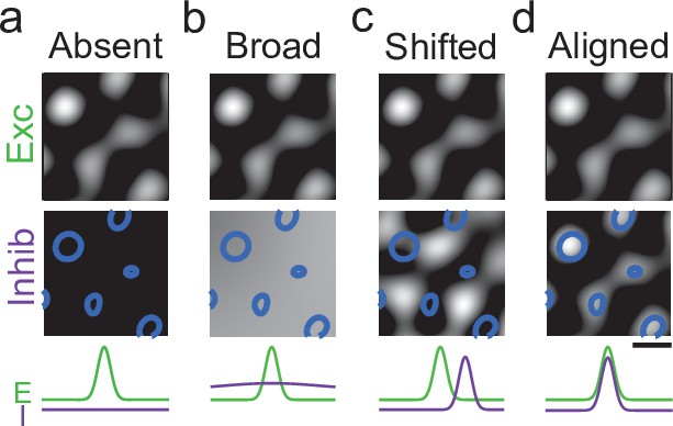
Possible modes of inhibition in the developing visual cortex.
Schematic showing potential arrangements of inhibitory and excitatory activity patterns in developing cortex. Top row: Excitation is known to be highly modular and spatially structured. Middle row: Inhibition could be absent (a), broadly unstructured (b), or modular (c, d); if modular, the spatial arrangement of those modules could be shifted with respect to excitatory activity (c), or already well aligned as found in the mature cortex (d). Scale bar: 1 mm.
Figure 2

GABAergic signaling has net inhibitory effect on cortical activity by P21.
(a) Experimental schematic; Ferret kits were injected with syn.GCaMP6s at approximately P10, and spontaneous activity was imaged at P21–23 (n=4 animals) both before and after bath application of the GABA antagonist bicuculine (BMI). (Right) Field-of-view for widefield epifluorescent calcium imaging. (b) Average trace across region of interest (ROI) for baseline spontaneous activity (top) and activity after BMI application (bottom) shows clear disinhibition of cortical activity. (c) Event frequency after BMI application is significantly higher than baseline (p<0.001; baseline=0.030 [0.016–0.050 ] Hz; BMI=0.200 [0.129–0.271 ] Hz; median, interquartile range [IQR], Wilcoxon rank-sum test). (d). Average event amplitude of BMI events are significantly higher than baseline (p<0.001; baseline=0.374 [0.190–0.535] ∆F/F, n (across four animals)=274 events; BMI=0.974 [0.470–1.220] ∆F/F, n=732 events; median, IQR, Wilcoxon rank-sum test).
-
Figure 2—source data 1
GABAergic signaling has net inhibitory effect on cortical activity by P21.
- https://cdn.elifesciences.org/articles/72456/elife-72456-fig2-data1-v1.pdf
Figure 3 with 2 supplements
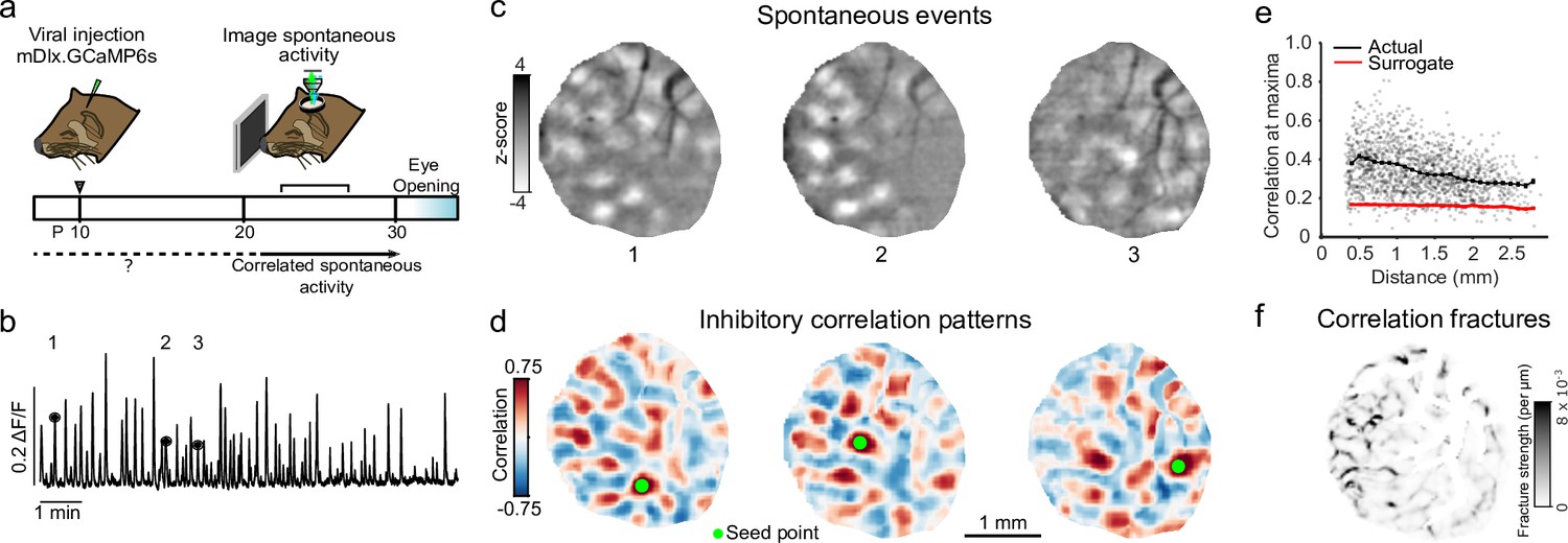
Spontaneous inhibitory activity is modular and participates in precisely organized large-scale correlated networks.
(a) Experimental schematic; ferret kits were injected with inhibitory specific mDlx.GCaMP6s at around P10, and spontaneous activity was imaged prior to eye-opening. (b) Example mean trace of inhibitory spontaneous activity across field of view for one representative animal. Numbers correspond to events in (c). (c) Example single-frame bandpass filtered events. (d) Spontaneous correlation patterns for three different seed points. (e) Correlation values at maxima as a function of distance from the seed point, as compared to surrogate shuffled correlations for the experiment shown in (b–d, f). (f) Fractures in correlation patterns reveal regions of rapid transition in global correlation structure.
Figure 3—figure supplement 1
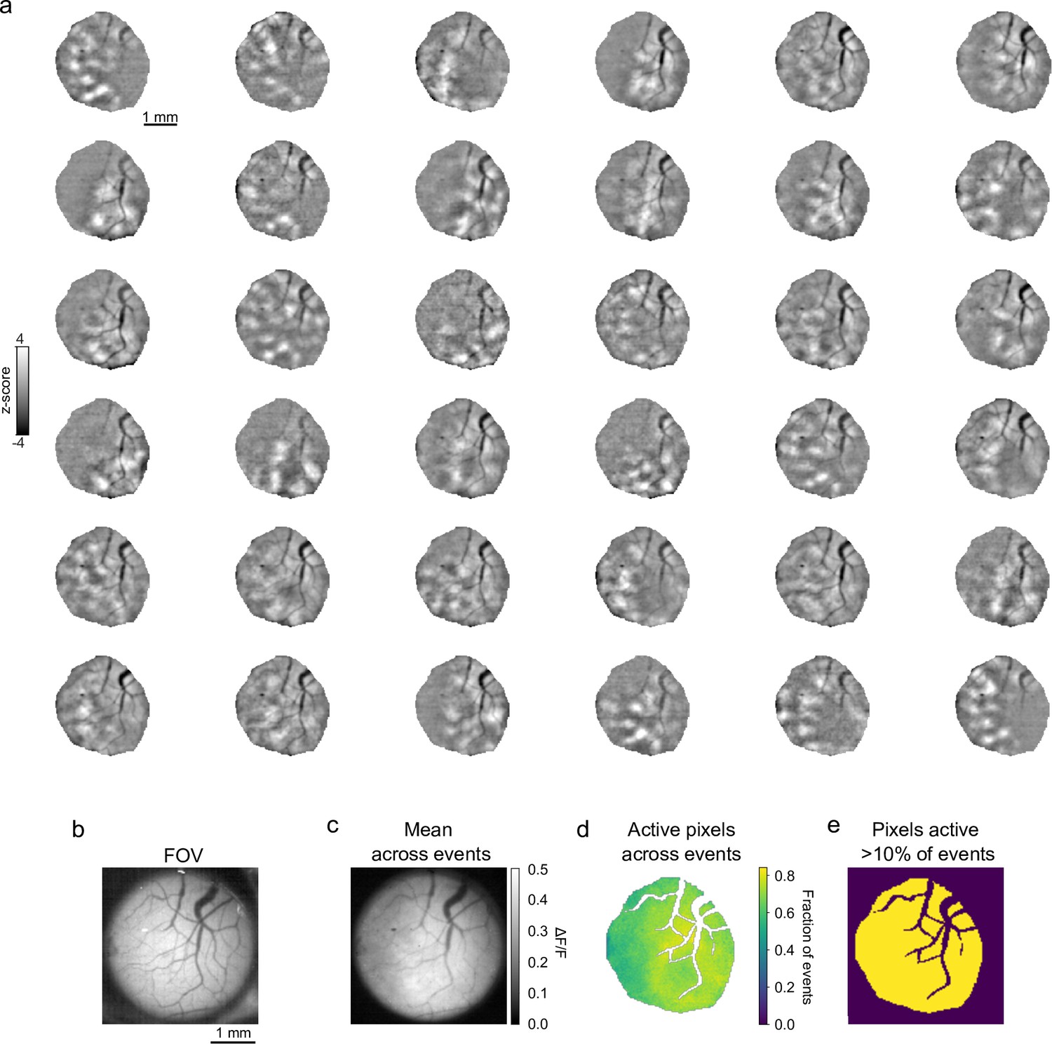
Spatial extent and variation of spontaneous inhibitory events.
Viral expression is robust and homogenous across our imaging area. (a) Thirty-six randomly selected spontaneous inhibition events, bandpass filtered. (b) Field-of-view (FOV) of cranial window for widefield calcium imaging. (c) Average ΔF/F across all events. (d) Percent of events where pixels within ROI were active (>3 s.d. over mean pixel activity) across all events (n=111). (e) All pixels within ROI participated in at least 10% of events. ROI, region of interest.
Figure 3—figure supplement 2
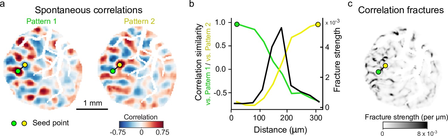
Correlation patterns of inhibitory spontaneous activity exhibit pronounced fractures.
(a) Example correlation patterns showing rapid change in correlation structure between nearby seed points (blood vessels masked). (b). Similarity of correlations falls off rapidly as the seed point is moved along the black line in (a), reflected in a sharp peak in fracture strength (per μm). (c). Spatial distribution of fracture strength for all pixels in ROI, showing seed points used in (a, b). Fracture image is reproduced from Figure 3f. ROI, region of interest.
Figure 4 with 1 supplement
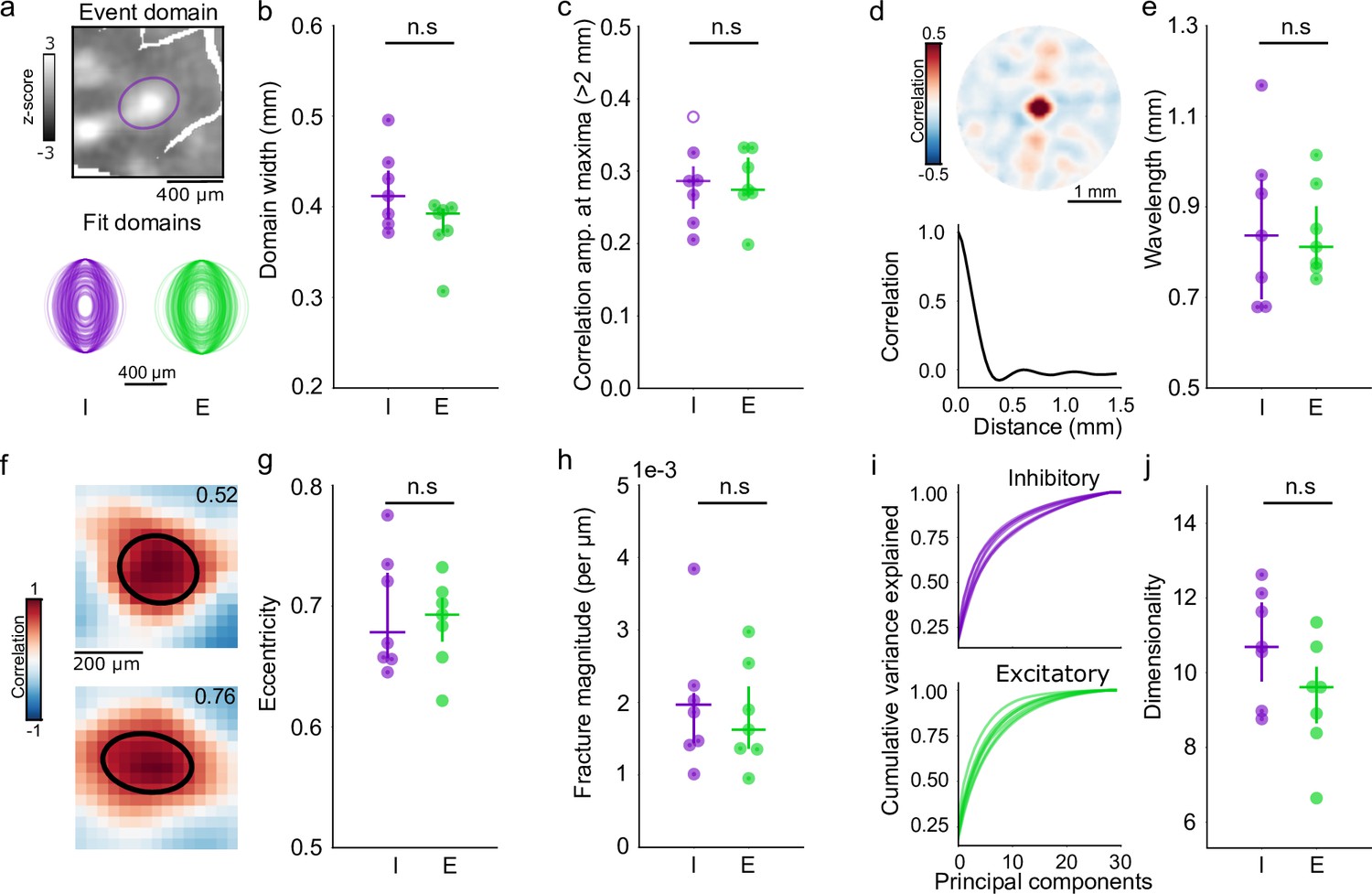
Quantitative agreement in structure of developing excitatory and inhibitory networks.
(a, b) Similar domain size for excitatory and inhibitory events. (a) Example event showing FWTM of Gaussian fit of active inhibitory domain (top) and fits of FWTM for 200 randomly selected domains from individual inhibitory (I, purple) and excitatory (E, green) animals, rotated to align major axis (bottom). (b) Median domain size for each I and E animal. Circles: individual animals, lines: group median and IQR. (c) Correlation strength at 1.8–2.2 mm from seed point. Filled circles individually significant versus surrogate (p<0.01). (d, e) Correlation wavelength is similar between I and E networks. (d) (top) Correlation pattern averaged over all seed points in single animal with inhibitory GCaMP. (bottom) Correlation as function of distance. (e). Wavelength of the correlation pattern for I and E. Circles: individual animals, lines: group median and IQR. (f–g) Similar eccentricity of local correlation structure. (f) Examples for two seed points from the same inhibitory animal, numbers indicate measured eccentricity. (g) Median eccentricity for all seed points. Circles: individual animals, lines: group median and IQR. (h) Fracture strength is similar for I and E networks. (i, j) Spontaneous activity is moderately low-dimensional in both E and I networks. (i) Cumulative explained variance for principal components of spontaneous events (lines indicate individual animals). (j). Median dimensionality, calculated from event-matched (n=30 events, n=100 simulations) random subsampling of events. Circles: individual animals, lines: group median and IQR. IQR, interquartile range.
Figure 4—figure supplement 1
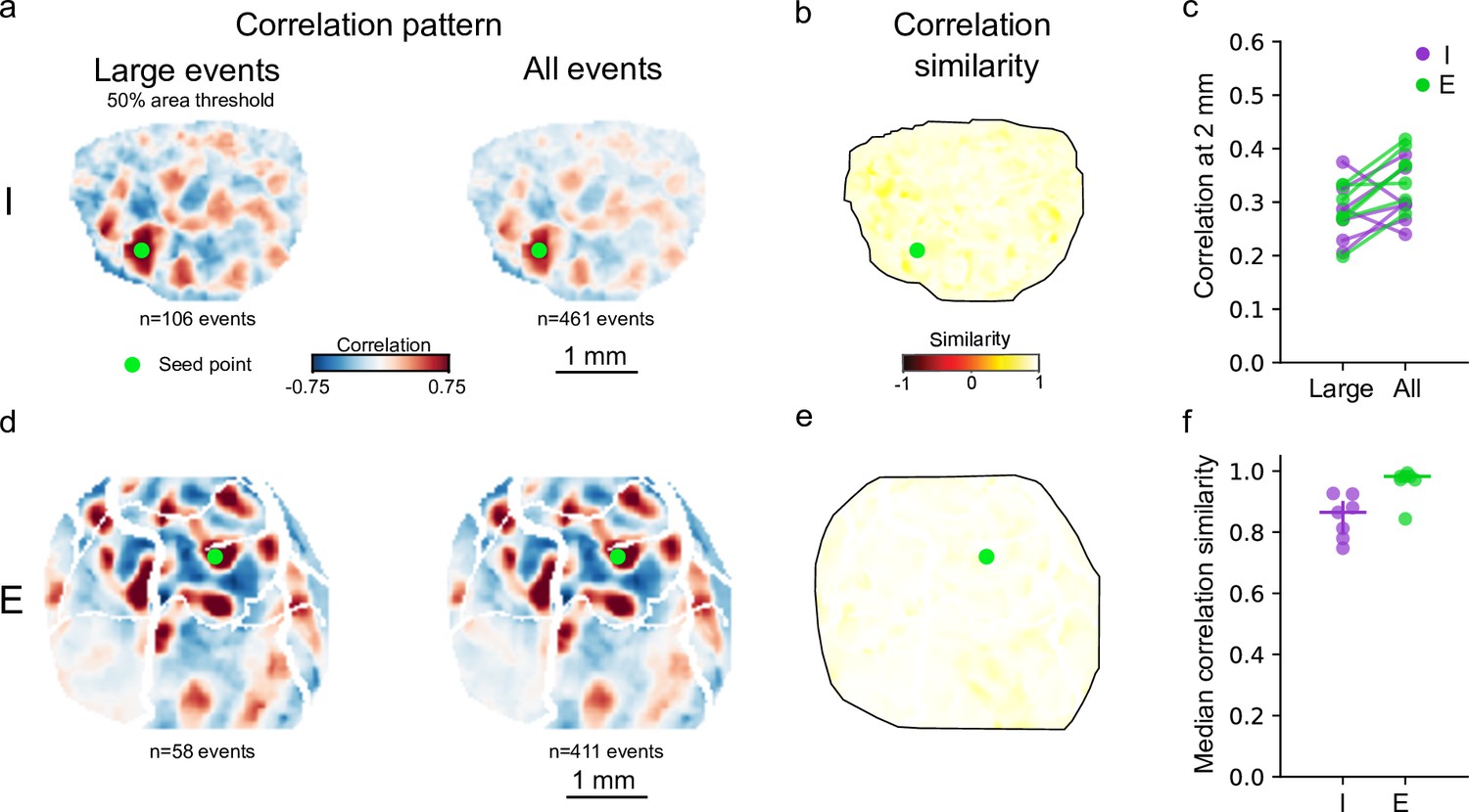
Spatial structure of inhibitory and excitatory correlation patterns from large events are highly similar to those computed from all events.
(a, d) Example inhibitory (a) and excitatory (d) correlation patterns generated using large events that extend over at least 50% of the ROI area (left, n=106 events) compared to patterns computed from all frames with active pixels (>3 s.d, 0% area threshold) (right, n=461 events). (b, e) Correlation similarity map comparing network made of Large events and network including All events (Large vs. All), for inhibitory (b) and excitatory (e) examples. (c). Strength of correlation maxima found 2 mm away from seed point for both inhibitory (I, purple) and excitatory (E, green) networks is not sensitive to area threshold. (f). Median value of Large versus All correlation similarity maps for all animals. Both inhibitory and excitatory networks show highly similar Large versus All correlation similarities, though excitatory similarities are greater than inhibitory (I: 0.87 [0.80–0.90], n=7. E: 0.98 [0.97–0.98],n=7, p=0.0088, Wilcoxon rank-sum test). ROI, region of interest.
Figure 5 with 1 supplement
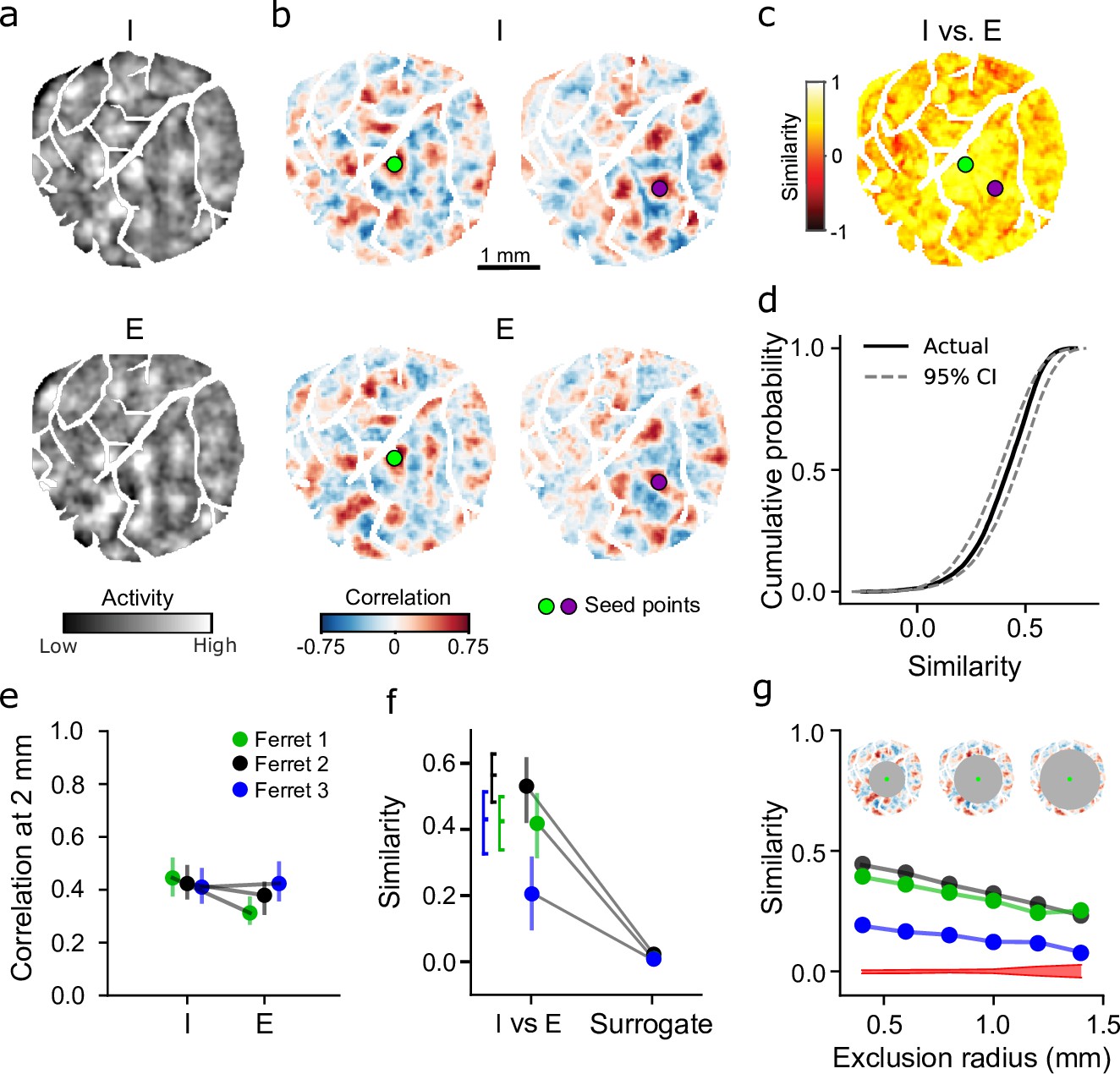
Inhibitory and excitatory networks show high degree of similarity within animal.
(a) Example spontaneous inhibitory (mDlx.GCaMP6s, top) and excitatory (syn.jRCaMP1a, bottom) events recorded from same animal (I color axis: –2 to –2 z-score, E color axis: –1 to 1 z-score). Example events were chosen based on pattern similarity. (b) Highly similar correlation patterns in inhibitory and excitatory networks for corresponding seed points. (c) Quantification of I versus E correlation similarity for all seed points. Circles indicate seed points illustrated in (b). (d). Similarity for all seed points in (c) falls within 95% confidence intervals (CIs) of bootstrapped I versus I similarity. (e) Within animal comparison of correlation strength for E and I (median and IQR within animal). Filled circles individually significant versus surrogate (p<0.01). (f) Similarity of I versus E correlations is significantly greater than shuffle (median and IQR within animal). Brackets indicate IQR of bootstrapped I versus I similarity. (g) Long-range correlations show significant network similarity. I versus E correlation similarity remains significant versus surrogate (red, 95% CI of surrogate, averaged across animals) for increasingly distant regions (excluding correlations within 0.4–1.4 mm from the seed point).
Figure 5—figure supplement 1
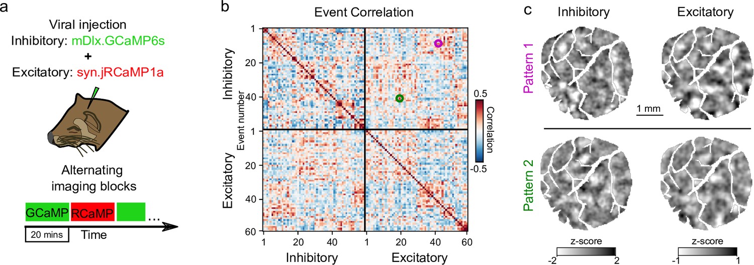
Similar patterns of spontaneous activity in inhibitory and excitatory events.
(a) Experimental schematic; I and E spontaneous activity imaged in interleaved 20 min blocks. (b) Sorted correlation matrix of inhibitory and excitatory events. Matrix shows not only clear clusters of repeating patterns within inhibitory and excitatory events, but also correlated patterns between inhibitory and excitatory events. Magenta and green circles indicate correlation value between example inhibitory and excitatory events in (c). (c) Example inhibitory and excitatory events with correlated spatial patterns.
Figure 6 with 3 supplements
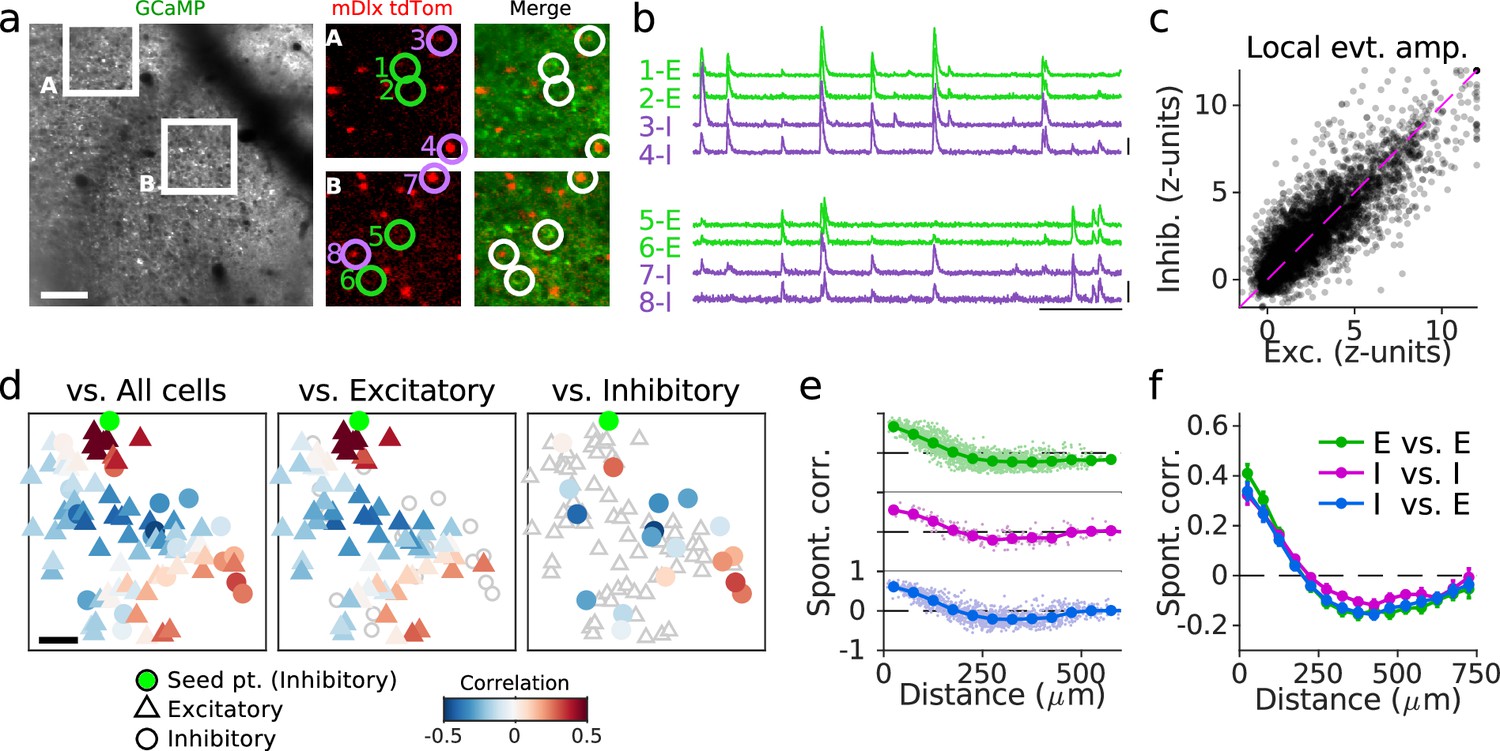
Cellular alignment of excitatory and inhibitory networks in developing visual cortex.
(a) (Left): Example FOV showing GCaMP signal from excitatory and inhibitory neurons. (Middle/Right): Expanded images showing nuclear tdTomato signal specifically in inhibitory neurons (middle) and merged with GCaMP signal (right). (b) Traces of spontaneous activity for excitatory (E, green) and inhibitory (I, purple) neurons as indicated in (a). (c). Event amplitude for local (<75 µm) excitatory and inhibitory responses. For clarity when plotting, 5% of responses are shown for 2186 cells and 1231 events from 21 FOV in five animals, and responses are clipped at 12 z-units. (d). Example pairwise correlations between an inhibitory neuron (green) and all cells (left), excitatory cells (middle), and inhibitory cells (right). (e). Pairwise correlations as function of distance for an example FOV shown in (a–d) for E-E, I-I, and E-I pairs. (f) same as (e) averaged over 21 FOV from five animals. Scale bars: (a, d): 100 µm; (b): 30 s, 3 ∆F/F. FOV, field-of-view.
Figure 6—figure supplement 1
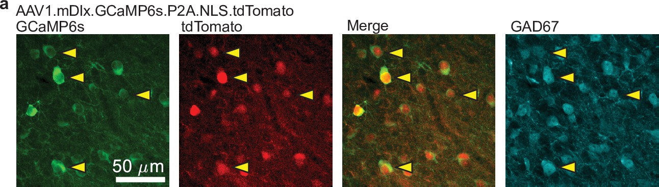
tdTomato expressed from AAV1.mDlx.GCaMP6s.P2A.NLS-tdTomato specifically labels GABAergic neurons.
(From left to right) Confocal images of GCaMP6s (green), tdTomato (red), merged GCaMP6s and tdTomato, and glutamate decarboxylase 67 (GAD67, cyan). Arrows indicate individual cell bodies, showing co-labeling of GCaMP6s, nuclear tdTomato, and GAD67.
Figure 6—figure supplement 2
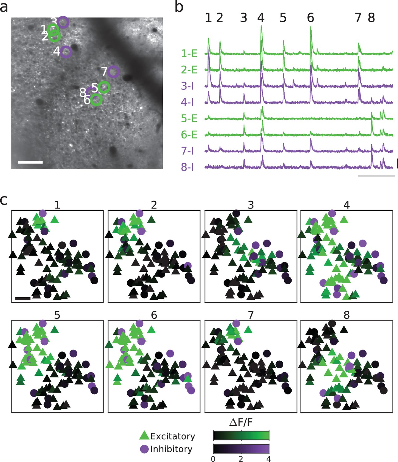
Spontaneous activity patterns are spatially modular and aligned across excitatory and inhibitory neurons.
(a, b) Example FOV and activity traces for excitatory and inhibitory neurons are shown in (a) (replotted from Figure 4). (c). Cellular activity patterns for eight spontaneous events are indicated in (b). Scale bars: (a, c): 100 µm; (b): 30 s, 3 ∆F/F. FOV, field-of-view.
Figure 6—figure supplement 3
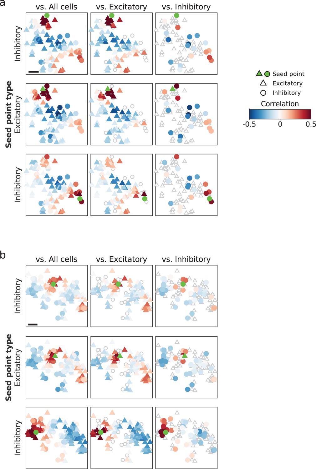
Examples of co-aligned correlation structure between excitatory and inhibitory cells.
(a) Top row: Pairwise correlations between an example inhibitory neuron and all cells (left), excitatory cells (middle), and inhibitory cells (right), replotted from Figure 4d. Middle and bottom row: additional example seed points (middle: excitatory neuron, bottom: inhibitory neuron) from same FOV. (b) same as (a), but for different animal. Scale bar: 100 μm. FOV, field-of-view.
Additional files
Download links
A two-part list of links to download the article, or parts of the article, in various formats.
Downloads (link to download the article as PDF)
Open citations (links to open the citations from this article in various online reference manager services)
Cite this article (links to download the citations from this article in formats compatible with various reference manager tools)
Tightly coupled inhibitory and excitatory functional networks in the developing primary visual cortex
eLife 10:e72456.
https://doi.org/10.7554/eLife.72456


