Phylogenomic analyses of echinoid diversification prompt a re-evaluation of their fossil record
- Department of Earth & Planetary Sciences, Yale University, United States
- Scripps Institution of Oceanography, University of California San Diego, United States
- Department of Earth Sciences, Natural History Museum, United Kingdom
- University College London Center for Life’s Origins and Evolution, United Kingdom
- Department of Invertebrate Zoology and Geology, California Academy of Sciences, United States
- Bader International Study Centre, Queen's University, Herstmonceux Castle, United Kingdom
- Departamento de Bioquímica y Biología Molecular, Facultad de Ciencias Biológicas, Universidad de Concepción, Chile
- School of Zoology, Faculty of Life Sciences, Tel Aviv University, Israel
- Steinhardt Museum of Natural History, Israel
- Department of Geology and Palaeontology, Natural History Museum Vienna, Austria
Figures
Figure 1
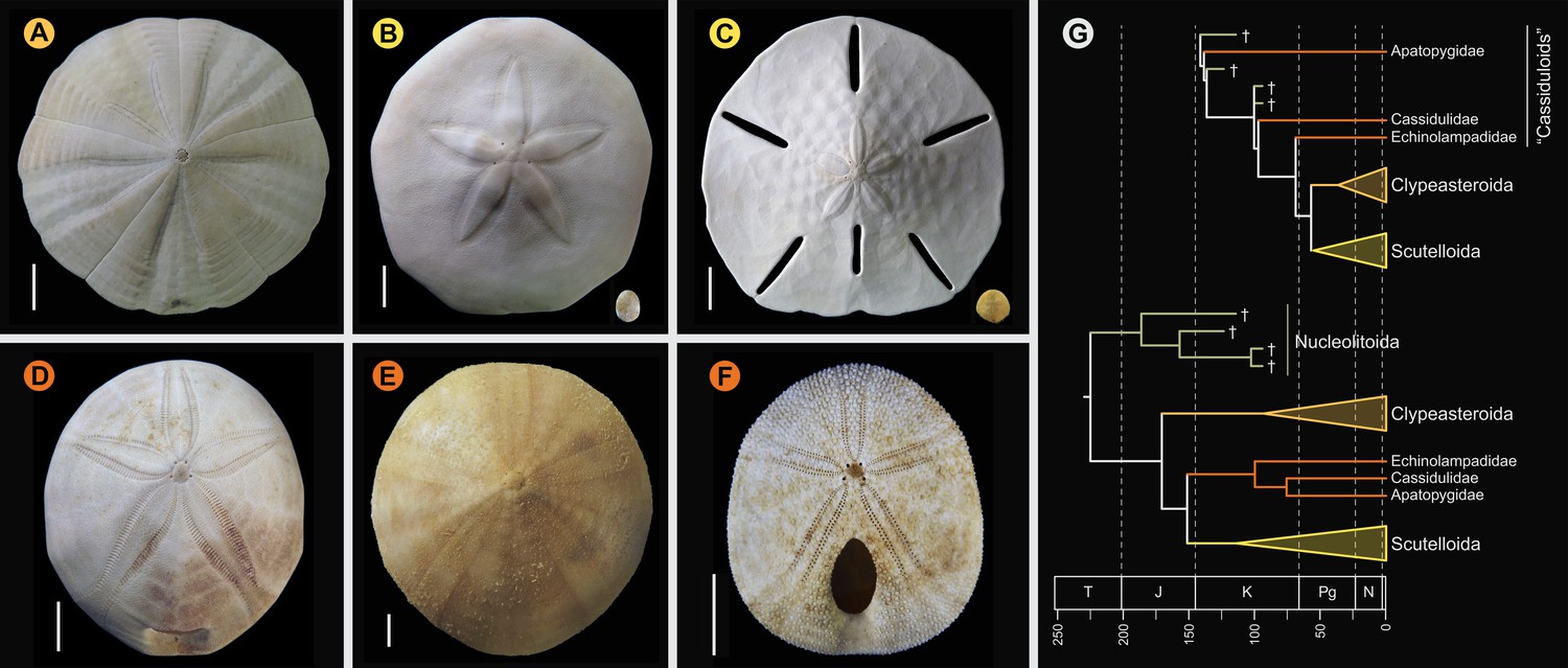
Neognathostomate diversity and phylogenetic relationships.
(A) Fellaster zelandiae, North Island, New Zealand (Clypeasteroida). (B) Large specimen: Peronella japonica, Ryukyu Islands, Japan; Small specimen: Echinocyamus crispus, Maricaban Island, Philippines (Laganina: Scutelloida). (C) Large specimen: Leodia sexiesperforata, Long Key, Florida; Small specimen: Sinaechinocyamus mai, Taiwan (Scutellina: Scutelloida). (D) Rhyncholampas pacificus, Isla Isabela, Galápagos Islands (Cassidulidae). (E) Conolampas sigsbei, Bimini, Bahamas (Echinolampadidae). (F)Apatopygus recens, Australia (Apatopygidae). (G) Hypotheses of relationships among neognathostomates. Top: Morphology supports a clade of Clypeasteroida + Scutelloida originating after the Cretaceous-Paleogene (K-Pg) boundary, subtended by a paraphyletic assemblage of extant (red) and extinct (green) ‘cassiduloids’ (Kroh and Smith, 2010). Bottom: A recent total-evidence study split cassiduloid diversity into a clade of extant lineages closely related to scutelloids, and an unrelated clade of extinct forms (Nucleolitoida; Mongiardino Koch and Thompson, 2021d). Divergence times are much older and conflict with fossil evidence. Cassidulids and apatopygids lacked molecular data in this analysis. Scale bars = 10 mm.
Figure 2
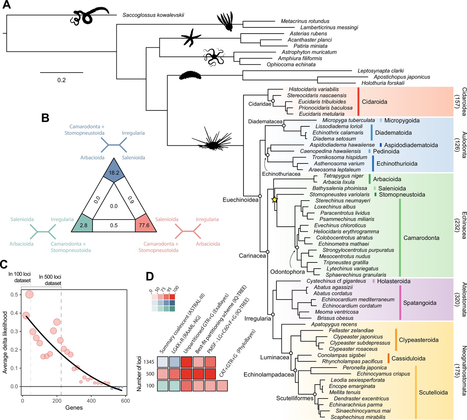
Phylogenetic relationships among major clades of Echinoidea.
(A) Favored topology, as obtained using the full supermatrix and a best-fit partitioning scheme in IQ-TREE (Nguyen et al., 2015). With the exception of a single contentious node within Echinacea (marked with a yellow star), all methods supported the same pattern of relationships, and assigned maximum support values to all nodes. Numbers below major clades correspond to the current numbers of described living species (obtained from Kroh and Mooi, 2020). (B) Likelihood-mapping analysis showing the proportion of quartets supporting different resolutions within Echinacea. While the majority of quartets support the topology depicted in A (shown in red), a relatively large number support an alternative resolution that has been recovered in morphological analyses (shown in blue; Kroh and Smith, 2010). (C) Difference in likelihood score (delta likelihood) for the two resolutions of Echinacea most strongly supported in the likelihood-mapping analysis. Genes were sorted based on their inferred phylogenetic usefulness (Mongiardino Koch, 2021b), and gene-wise delta scores were averaged for datasets composed of multiples of 20 loci. Support for a clade of Salenioida + (Camarodonta + Stomopneustoida), as depicted in A, is seen as positive delta scores and is predominantly concentrated among the most phylogenetically useful loci. This signal is attenuated in larger datasets that contain less reliable genes, eventually favoring an alternative resolution (as seen by negative scores for the largest datasets). Only the 584 loci containing data for the three main lineages of Echinacea were considered. The line corresponds to a second-degree polynomial regression. (D) Resolution and bootstrap scores (see color scale) of the topology within Echinacea found using datasets of different sizes and alternative methods of inference.
Figure 3

Estimated branch lengths across different models of molecular evolution.
Different site-homogeneous models (left) infer similar levels of divergence, and the choice between them induces little distortion in the general tree structure. Site-heterogeneous models on the other hand not only infer a larger degree of divergence between terminals relative to site-homogeneous ones (center and right), but they also distort the tree (i.e., impose a non-isometric stretching), with branch lengths connecting outgroup taxa expanding much more than those within the ingroup clade.
Figure 4 with 1 supplement
The 10 most sensitive node dates are found within Cidaroidea, Aulodonta, Neognathostomata, and among outgroup nodes.
For each, the range shown spans the interval between the minimum and maximum ages found among the consensus topologies of the 80 time-calibrated runs performed.
Figure 4—figure supplement 1
Median ages for selected clades across the consensus trees of the 80 time-calibrated experiments performed.
Figure 5 with 5 supplements
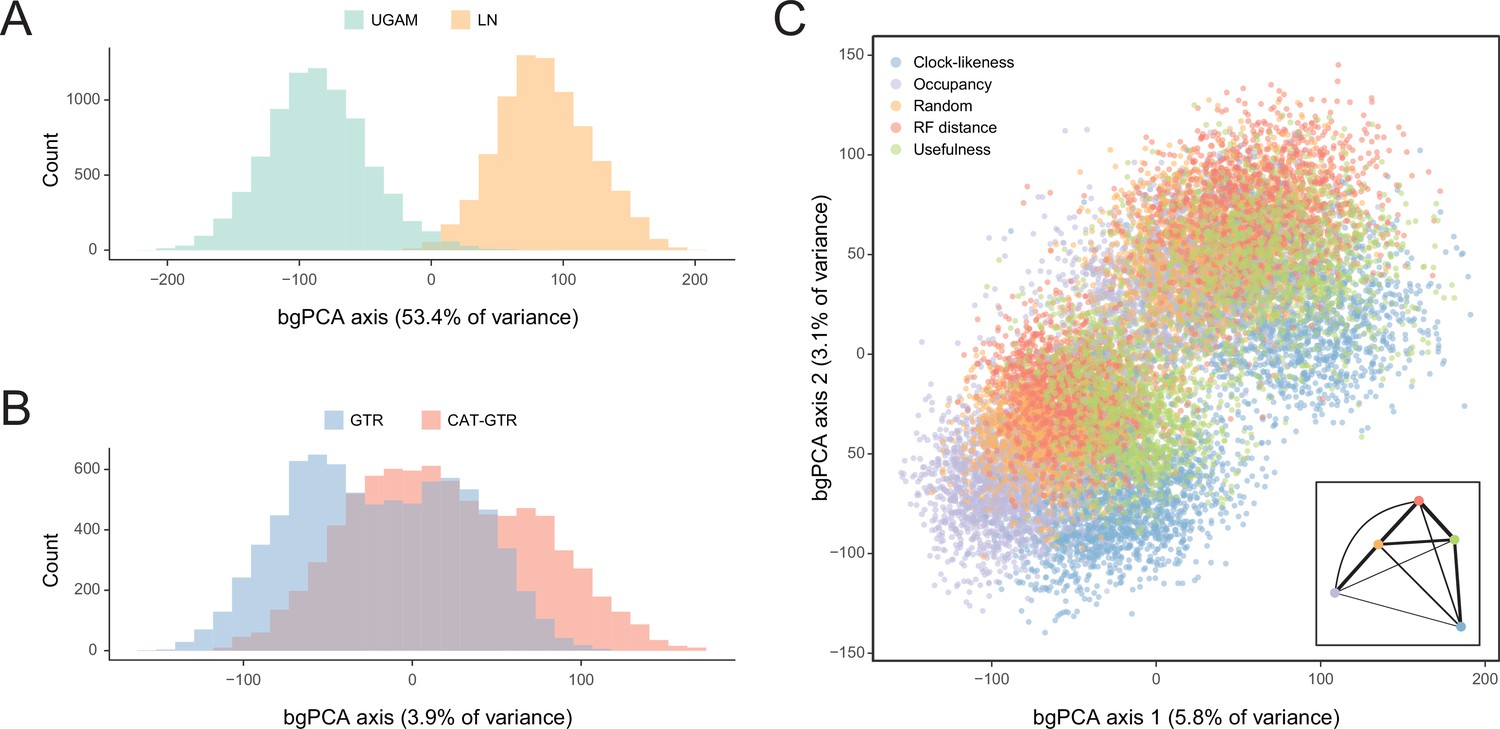
Sensitivity of divergence time estimation to methodological decisions.
Between-group principal component analysis (bgPCA) was used to retrieve axes that separate chronograms based on the clock model (A), model of molecular evolution (B), and gene sampling strategy (C) employed. In the latter case, only the first two out of four bgPCA dimensions are shown. The inset shows the centroid for each loci sampling strategy, and the width of the lines connecting them are scaled to the inverse of the Euclidean distances that separates them (as a visual summary of overall similarity). The proportions of total variance explained are shown on the axis labels. The impact of the clock model is such that a bimodal distribution of chronograms can be seen even when bgPCA are built to discriminate based on other factors (as in C).
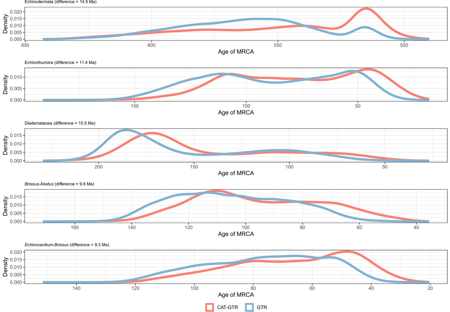
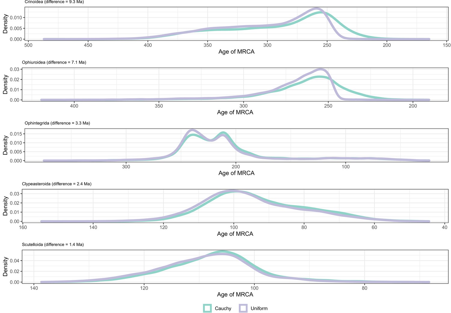
Figure 5—figure supplement 1
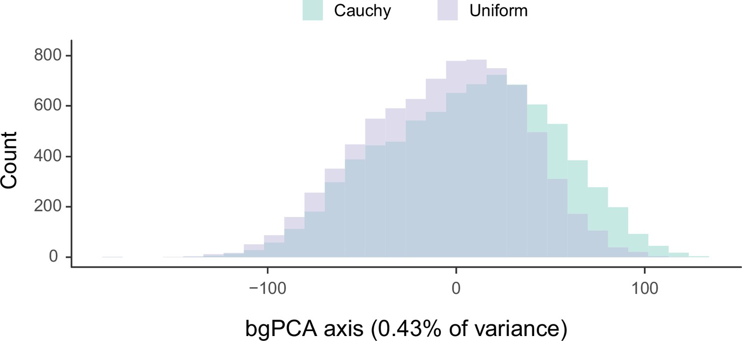
Sensitivity of divergence time estimation to the use of alternate prior distributions on calibrated nodes.
Between-group principal component analysis (bgPCA) was used to retrieve the axes of maximum discrimination between chronograms estimated by enforcing either uniform or Cauchy prior distributions. The proportion of total variance explained by this axis is shown on the label.
Figure 5—figure supplement 2
Distribution of posterior probabilities for node ages that show an average difference larger than 20 Myr depending on the choice of clock prior.
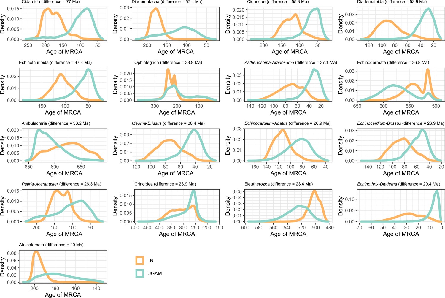
Figure 5—figure supplement 3
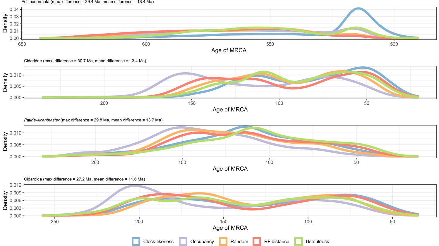
Distribution of posterior probabilities for node ages that show a maximum difference larger than 20 Myr depending on the gene sampling strategy.
The largest differences can be seen in the relatively younger ages of Ambulacraria and Echinodermata when using clock-like genes, and in the relatively older ages for some nodes within cidaroids and asteroids when using loci with high occupancy. Other sampling criteria largely agree on inferred node ages, as can also be seen in Figure 5C as short distances between their centroids in the chronospace.
Figure 5—figure supplement 4
Distribution of posterior probabilities for node ages that are the most affected by the choice of model of molecular evolution.
No node showed average differences larger than 20 Myr, so those suffering the biggest changes are shown instead.
Figure 5—figure supplement 5
Distribution of posterior probabilities for node ages that are the most affected by the choice of prior distributions on calibrated nodes.
No node showed average differences larger than 20 Myr, so those suffering the biggest changes are shown instead.
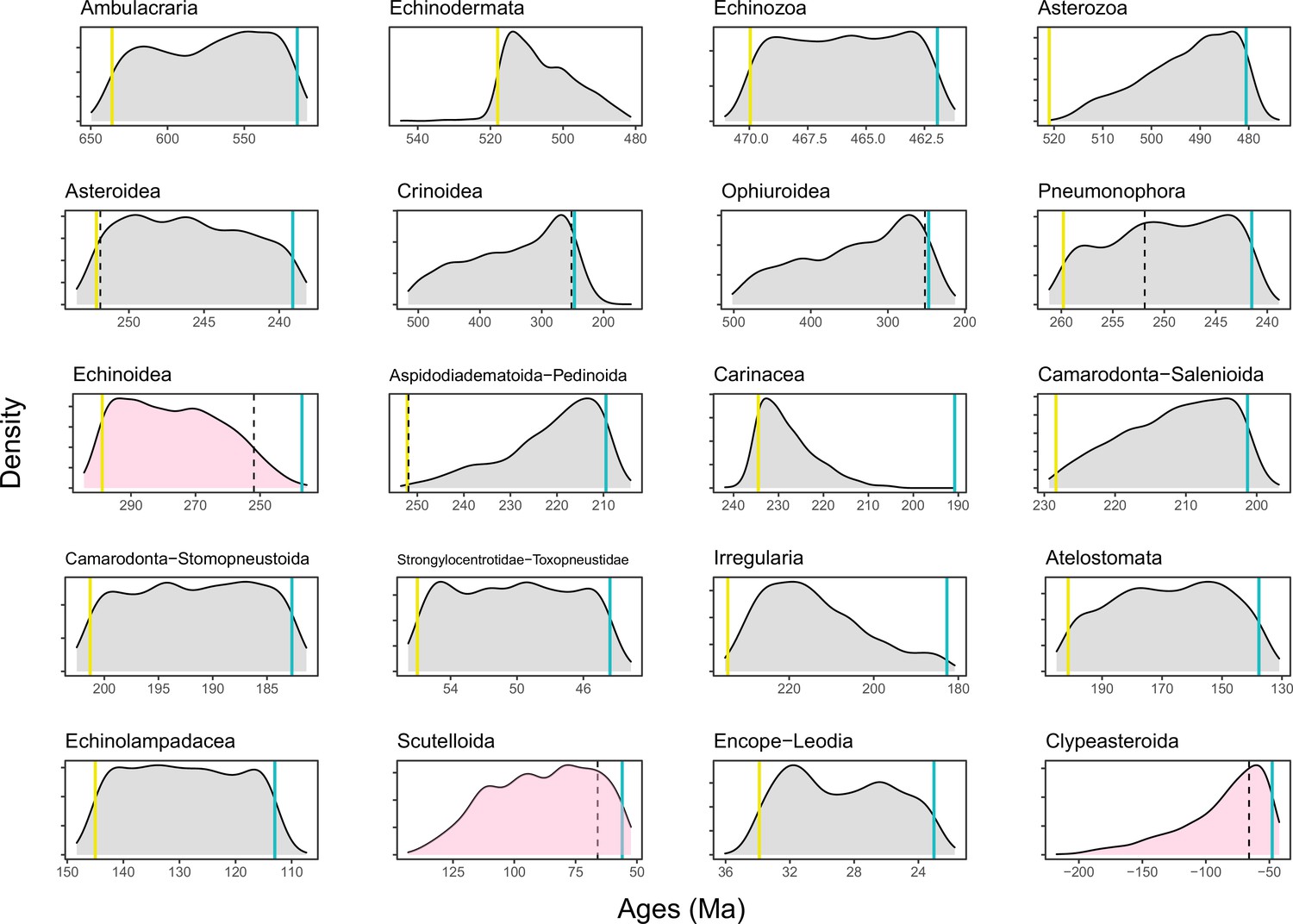
Figure 6 with 2 supplements
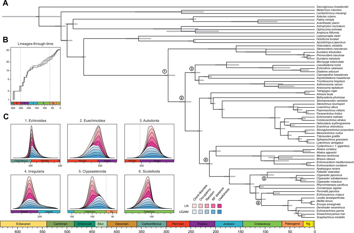
Divergence times among major clades of Echinoidea and other echinoderms.
(A) Consensus chronogram of the two PhyloBayes (Lartillot et al., 2013) runs using clock-like genes under a CAT + GTR + G model of evolution, an autocorrelated log-normal (LN) clock, and Cauchy prior distributions. Node ages correspond to median values, and bars show the 95% highest posterior density intervals. (B) Lineage-through-time plot, showing the rapid divergence of higher-level clades following the P-T mass extinction (shown with dashed lines, along with the Cretaceous-Paleogene [K-Pg] boundary). Each line corresponds to an individual consensus topology from among the 80 time-calibrated runs performed. (C) Posterior distributions of the ages of selected nodes (identified in A with numbers). The effects introduced by the use of different models of molecular evolution and node age prior distributions are not shown, as they represent the least important factors (see Figure 5); the posterior distributions obtained under different settings of these were merged for every combination of targeted loci and clock prior. Tick marks = 10 Myr.
Figure 6—figure supplement 1
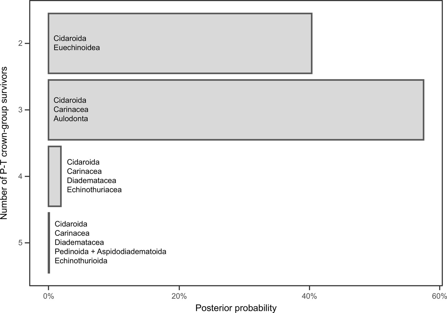
Number of lineages inferred to have crossed the Permian-Triassic (P-T) boundary.
The probabilities of each scenario are estimated from the inferred divergence times of the 16,000 chronograms sampled across all of the analyses performed (200 for the two runs of each combination of sampled loci, model of molecular evolution, and clock model and prior distribution on node ages). The probability of three or more crown group lineages surviving the P-T extinction is 59.58%. Names show the combination of clades crossing the P-T boundary for each scenario of number of survivors.
Figure 6—figure supplement 2
Prior distributions of all constrained nodes.
Five-hundred replicates were sampled from the joint prior, showing appropriately broad distributions of node ages. Blue lines show minima and yellow ones maxima (when enforced); dotted lines show the age of the Permian-Triassic (251.9 Ma) and Cretaceous-Paleogene (66 Ma) mass extinction events. Nodes whose ages are of special interest (Echinoidea, Scutelloida, and Clypeasteroida) are shown in pink, revealing large prior probabilities of the divergence occurring at either side of mass extinction events.
Figure 7
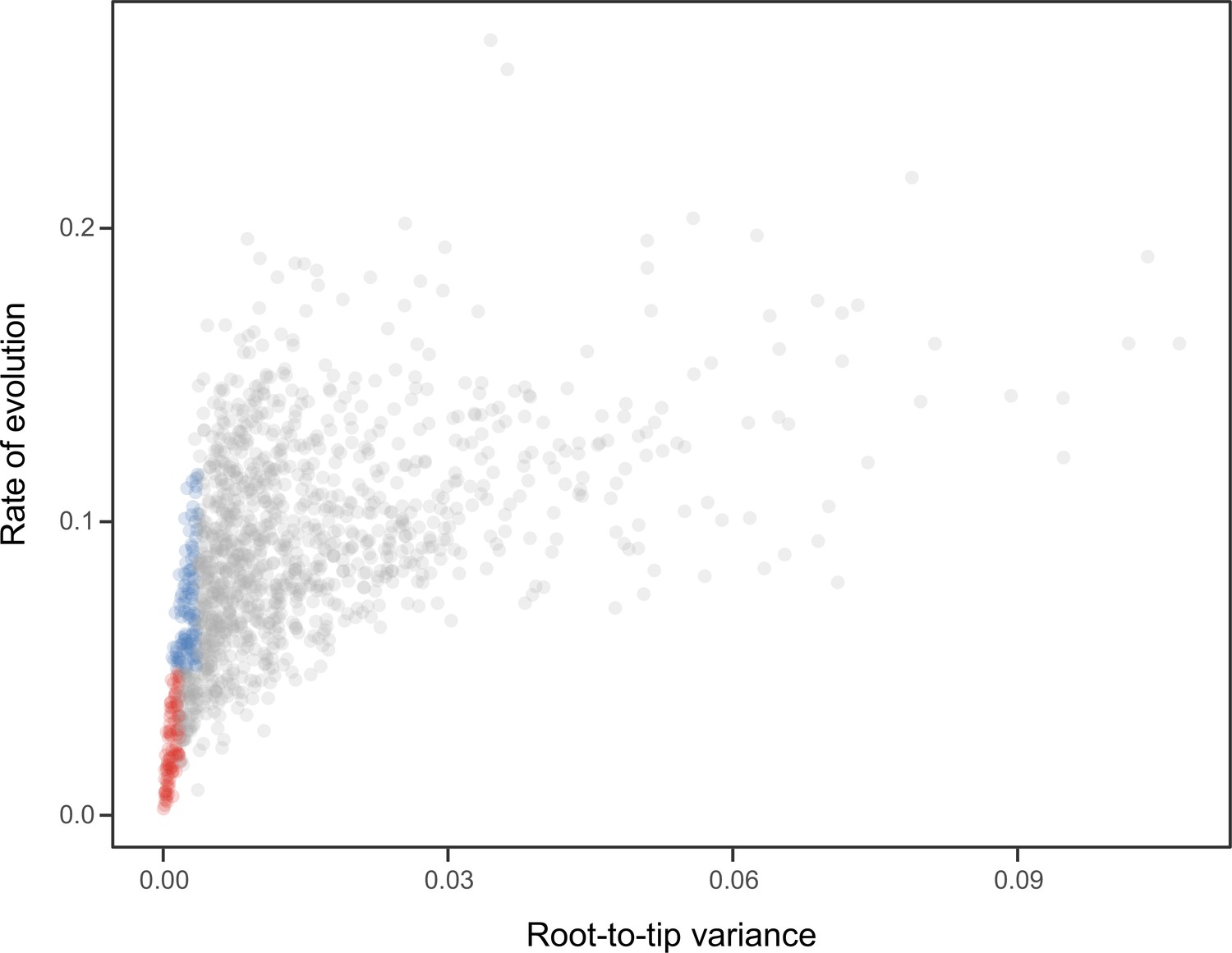
Relationship between the root-to-tip variance (a proxy for the clock-likeness of loci) and the rate of evolution.
The most clock-like loci (shown in red), which are often favored for the inference of divergence times (e.g., Smith et al., 2018; Carruthers et al., 2020), are among the most highly conserved and can provide little information for constraining node ages (see also Mongiardino Koch, 2021b). Clock-like genes with a higher information content were used instead by choosing the loci with the lowest root-to-tip variance from among those that were within one standard deviation from the mean evolutionary rate (shown in blue).
Appendix 3—figure 1

Ordering of loci enforced using genesortR (Mongiardino Koch, 2021b) and its relationship to the seven gene properties employed.
High ranking loci (i.e., the most phylogenetically useful) show low root-to-tip variances (or high clock-likeness), low saturation, and low compositional heterogeneity, as well as high average bootstrap and Robinson-Foulds similarity to a target topology (in this case, with the contentious relationship among major lineages of Echinacea collapsed).
Appendix 3—figure 2
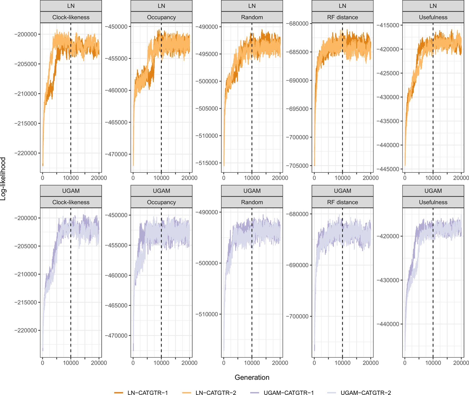
Trace plots of the log-likelihood of different time calibration runs.
All runs show evidence of reaching convergence and stationarity before our imposed burn-in fraction of 10,000 generations (dashed lines). For simplicity, only runs under the CAT + GTR + G model and Cauchy priors are plotted. Those run under uniform node age priors behaved identically, while those run under GTR + G converged much faster.
Tables
Appendix 1—table 1
Transcriptomic/genomic datasets added in this study relative to the taxon sampling of Mongiardino Koch et al., 2018 and Mongiardino Koch and Thompson, 2021d.
Taxa with citations were taken from the literature, and details can be found in the corresponding studies and associated NCBI BioProjects. Taxa are shown in alphabetical order; those identified with ‘OG’ are outgroup taxa (i.e., non-echinoids). Voucher specimens are deposited at the Benthic Invertebrate Collection, Scripps Institution of Oceanography (SIO-BIC), and the Echinoderm Collection, Muséum National d’Histoire Naturelle (MNHN-IE). If multiple accession numbers are shown for a given taxon, these datasets were merged before assembly. Similar details for all other specimens can be found in Mongiardino Koch et al., 2018 and Mongiardino Koch and Thompson, 2021d.
| Taxon | Citation | Tissue type | Collector | Locality (depth) | Voucher | GenBank accession number |
|---|---|---|---|---|---|---|
| Amphiura filiformis (OG) | Dylus et al., 2016 | – | – | – | – | SRX2255774 |
| Apatopygus recens | This study | Mixed | Owen Anderson | Foveaux Strait, South Island, New Zealand | SIO-BIC E7142 | SRR16134561 |
| Aspidodiadema hawaiiense | This study | Mixed | Greg Rouse, Avery Hiley | Seamount 4, Costa Rica, Pacific Ocean (1003 m) | SIO-BIC E7363 | SRR16134560 |
| Asterias rubens (OG) | Reich et al., 2015 | – | – | – | – | SRX445860 |
| Astrophyton muricatum (OG) | Janies et al., 2016; Linchangco et al., 2017 | – | – | – | – | SRX1391908 |
| Bathysalenia phoinissa | This study | Tube feet, spine muscles | BIOMAGLO Cruise Team | Mozambique Channel, Mayotte (295–336 m) | MNHN-IE-2016–23 | SRR15130003 |
| Clypeaster japonicus | This study | Eggs | Frances Armstrong | Misaki Marine Biological Station, Kanagawa, Japan | – | SRR16134552 |
| Echinothrix calamaris | This study | Male gonad | – | Philippines | – | SRR16134551 |
| Encope emarginata | This study | Eggs | Gulf Specimen Marine Lab | Apalachee Bay, FL, USA | – | SRR16134550 |
| Eucidaris metularia | This study | Mixed | Greg Rouse | Al-Fahal Reef, Red Sea, Makkah, Saudi Arabia | SIO-BIC 2017–008 | SRR16134549 |
| Fellaster zelandiae | This study | Spines, tube feet, gut, joining tissue of Aristotle’s lantern | Wilma Blom | Western end of Cornwallis Beach, Auckland, New Zealand | SIO-BIC E7920 | SRR16134548 |
| Histocidaris variabilis | This study | Gonad | Greg Rouse, Avery Hiley | Las Gemelas Seamount, near Isla del Coco, Costa Rica, Pacific Ocean (571 m) | SIO-BIC E7350 | SRR16134547 |
| Lamberticrinus messingi (OG) | Clouse et al., 2015; Janies et al., 2016 | – | – | – | – | SRX1397823 |
| Leodia sexiesperforata | This study | Eggs | Frances Armstrong | Bocas del Toro, Panama | – | SRR16134546 |
| Metacrinus rotundus (OG) | Koga et al., 2016 | – | – | – | – | DRX021520 |
| Micropyga tuberculata | This study | Tube feet, spine muscles | BIOMAGLO Cruise Team | Mozambique Channel, Îles Glorieuses (385–410 m) | MNHN-IE-2016–39 | SRR15130004 |
| Ophiocoma echinata (OG) | Reich et al., 2015 | – | – | – | – | SRX445856 |
| Peronella japonica | This study | Eggs | Frances Armstrong | Kanazawa, Japan | – | SRR16134545 |
| Rhyncholampas pacificus | This study | Mixed | Carlos A. Conejeros-Vargas | Panteón Beach, Puerto Ángel Bay, Oaxaca, Mexico | SIO-BIC E7918 | SRR16134558 |
| Scaphechinus mirabilis | Simakov et al., 2015 | – | – | – | – | DRX187887 DRX187888 |
| Sinaechinocyamus mai | This study | Gregory’s diverticulum | Jih-Pai Lin | Miaoli County, Taiwan | SIO-BIC E7919 | SRR16134557 |
| Sterechinus neumayeri | Collins et al., 2021 | – | – | – | – | ERX3498697 ERX3498698 ERX3498699 ERX3498700 ERX3498701 |
| Stereocidaris nascaensis | This study | Muscle surrounding Aristotle’s lantern | Charlotte Seid | Off San Ambrosio, Desventuradas Islands, Chile (215 m) | SIO-BIC E7154 | SRR16134559 |
| Tetrapygus niger | This study | Female gonad, tube feet | Felipe Aguilera | Dichato Bay, Chile | – | SRR16134553 SRR16134554 |
| Tripneustes gratilla | This study | Pedicellariae | – | Philippines | – | SRR16134556 |
| Tromikosoma hispidum | This study | Tube feet | Lisa Levin, Todd Litke | Quepos Plateau, Costa Rica, Pacific Ocean (2067 m) | SIO-BIC E7251 | SRR16134555 |
Appendix 1—table 2
Details of molecular datasets and supermatrix.
Statistics for raw reads and assemblies are shown for datasets incorporated in this study relative to the sampling of Mongiardino Koch et al., 2018 and Mongiardino Koch and Thompson, 2021d, where similar statistics can be found for the other datasets. Taxa are shown in alphabetical order; those identified with ‘OG’ are outgroup taxa (i.e., non-echinoids). Novel datasets correspond to Illumina pair-end transcriptomes, except for two draft genomes (Bathysalenia phoinissa and Micropyga tuberculata). Mean insert size is expressed in number of base pairs. For transcriptomes, read pairs (initial) shows numbers input into Agalma (Dunn et al., 2013), that is, after processing with Trimmomatic (Bolger et al., 2014) or UrQt (Modolo and Lerat, 2015), while read pairs (retained) show those that passed the Agalma curation checks (including ribosomal, adapter, quality, and compositional filters), and represent the final number of read pairs used for assembly. For genomes, see information in the bioinformatic details above. Assemblies were further sanitized with either alien_index (Ryan, 2014) alone or in combination with CroCo (Simion et al., 2018), and the number of assembled transcripts/contigs shows the size of datasets after these curation steps. The number of loci shows the occupancy of terminals in the supermatrix output by Agalma (1346 loci at 70% occupancy), after which loci were further removed by TreeShrink (Mai and Mirarab, 2018), resulting in the final occupancy scores.
| Species | Mean insert size | Read pairs (initial) | Read pairs (retained) | Assembled transcripts/contigs | Number of loci | Removed by TreeShrink | Final occupancy |
|---|---|---|---|---|---|---|---|
| Abatus agassizii | – | – | – | – | 522 | 5 | 38.4 |
| Abatus cordatus | – | – | – | – | 497 | 2 | 36.8 |
| Acanthaster planci (OG) | – | – | – | – | 864 | 8 | 63.6 |
| Amphiura filiformis (OG) | 180.1 | 61,558,173 | 52,206,727 | 416,946 | 761 | 8 | 55.9 |
| Apatopygus recens | 415.3 | 74,315,687 | 56,898,850 | 274,380 | 1152 | 5 | 85.2 |
| Apostichopus japonicus (OG) | – | – | – | – | 849 | 9 | 62.4 |
| Araeosoma leptaleum | – | – | – | – | 1184 | 2 | 87.8 |
| Arbacia lixula | – | – | – | – | 1234 | 1 | 91.6 |
| Aspidodiadema hawaiiense | 228.7 | 109,716,219 | 104,518,714 | 311,032 | 1060 | 11 | 77.9 |
| Asterias rubens (OG) | 230.4 | 31,890,613 | 25,495,009 | 103,090 | 805 | 9 | 59.1 |
| Asthenosoma varium | – | – | – | – | 1254 | 7 | 92.6 |
| Astrophyton muricatum (OG) | 195.9 | 25,191,954 | 22,281,829 | 149,146 | 478 | 5 | 35.1 |
| Bathysalenia phoinissa | – | – | – | 154,120 | 605 | 6 | 44.5 |
| Brissus obesus | – | – | – | – | 773 | 0 | 57.4 |
| Caenopedina hawaiiensis | – | – | – | – | 1094 | 2 | 81.1 |
| Clypeaster japonicus | 198.6 | 10,505,520 | 9,298,316 | 74,743 | 829 | 1 | 61.5 |
| Clypeaster rosaceus | – | – | – | – | 1242 | 2 | 92.1 |
| Clypeaster subdepressus | – | – | – | – | 1233 | 3 | 91.4 |
| Colobocentrotus atratus | – | – | – | – | 1158 | 0 | 86.0 |
| Conolampas sigsbei | – | – | – | – | 1001 | 5 | 74.0 |
| Cystechinus c.f. giganteus | – | – | – | – | 661 | 0 | 49.1 |
| Dendraster excentricus | – | – | – | – | 337 | 1 | 25.0 |
| Diadema setosum | – | – | – | – | 305 | 1 | 22.6 |
| Echinarachnius parma | – | – | – | – | 1187 | 3 | 88.0 |
| Echinocardium cordatum | – | – | – | – | 1012 | 2 | 75.0 |
| Echinocardium mediterraneum | – | – | – | – | 1185 | 1 | 88.0 |
| Echinocyamus crispus | – | – | – | – | 709 | 6 | 52.2 |
| Echinometra mathaei | – | – | – | – | 1055 | 0 | 78.4 |
| Echinothrix calamaris | 203.9 | 68,871,087 | 60,443,904 | 251,788 | 1252 | 4 | 92.7 |
| Encope emarginata | 206.2 | 12,015,888 | 10,461,870 | 66,241 | 1076 | 1 | 79.9 |
| Eucidaris metularia | 321.6 | 38,802,159 | 29,047,401 | 83,318 | 412 | 2 | 30.5 |
| Eucidaris tribuloides | – | – | – | – | 414 | 0 | 30.8 |
| Evechinus chloroticus | – | – | – | – | 1196 | 1 | 88.8 |
| Fellaster zelandiae | 313.9 | 62,619,791 | 51,742,748 | 168,598 | 1269 | 1 | 94.2 |
| Heliocidaris erythrogramma | – | – | – | – | 931 | 0 | 69.2 |
| Histocidaris variabilis | 329.2 | 84,103,672 | 73,884,180 | 144,044 | 1189 | 5 | 88.0 |
| Holothuria forskali (OG) | – | – | – | – | 743 | 8 | 54.6 |
| Lamberticrinus messingi (OG) | 195.0 | 22,989,820 | 20,234,597 | 59,049 | 351 | 3 | 25.9 |
| Leodia sexiesperforata | 203.8 | 16,211,182 | 14,174,475 | 68,964 | 1064 | 1 | 79.0 |
| Leptosynapta clarki (OG) | – | – | – | – | 403 | 4 | 29.6 |
| Lissodiadema lorioli | – | – | – | – | 770 | 0 | 57.2 |
| Loxechinus albus | – | – | – | – | 1265 | 1 | 93.9 |
| Lytechinus variegatus | – | – | – | – | 1257 | 2 | 93.2 |
| Mellita tenuis | – | – | – | – | 1002 | 1 | 74.4 |
| Meoma ventricosa | – | – | – | – | 1053 | 0 | 78.2 |
| Mesocentrotus nudus | – | – | – | – | 1247 | 0 | 92.6 |
| Metacrinus rotundus (OG) | 198.5 | 23,791,832 | 20,900,345 | 83,718 | 642 | 7 | 47.2 |
| Micropyga tuberculata | – | – | – | 170,514 | 415 | 4 | 30.5 |
| Ophiocoma echinata (OG) | 278.5 | 28,427,026 | 24,836,025 | 130,153 | 712 | 7 | 52.4 |
| Paracentrotus lividus | – | – | – | – | 1266 | 0 | 94.1 |
| Patiria miniata (OG) | – | – | – | – | 740 | 8 | 54.4 |
| Peronella japonica | 208.3 | 17,696,287 | 15,707,931 | 106,110 | 1043 | 6 | 77.0 |
| Prionocidaris baculosa | – | – | – | – | 794 | 3 | 58.8 |
| Psammechinus miliaris | – | – | – | – | 1173 | 1 | 87.1 |
| Rhyncholampas pacificus | 346.8 | 63,116,413 | 52,160,741 | 234,910 | 1070 | 2 | 79.3 |
| Saccoglossus kowalevskii (OG) | – | – | – | – | 668 | 6 | 49.2 |
| Scaphechinus mirabilis | 401.7 | 10,169,195 | 8,796,067 | 127,664 | 974 | 4 | 72.1 |
| Sinaechinocyamus mai | 297.2 | 60,208,172 | 52,265,201 | 164,646 | 1233 | 1 | 91.5 |
| Sphaerechinus granularis | – | – | – | – | 1214 | 1 | 90.1 |
| Sterechinus neumayeri | 207.3 | 26,376,279 | 21,308,840 | 122,001 | 1097 | 1 | 81.4 |
| Stereocidaris nascaensis | 327.0 | 69,962,495 | 60,316,050 | 121,508 | 1200 | 6 | 88.7 |
| Stomopneustes variolaris | – | – | – | – | 908 | 0 | 67.5 |
| Strongylocentrotus purpuratus | – | – | – | – | 1266 | 5 | 93.7 |
| Tetrapygus niger | 202.5 | 63,040,541 | 52,761,671 | 163,084 | 1287 | 2 | 95.5 |
| Tripneustes gratilla | 154.6 | 62,962,239 | 57,015,692 | 130,376 | 1309 | 1 | 97.2 |
| Tromikosoma hispidum | 300.4 | 57,208,357 | 47,909,038 | 234,502 | 1238 | 7 | 91.5 |
Additional files
Download links
A two-part list of links to download the article, or parts of the article, in various formats.
Downloads (link to download the article as PDF)
Open citations (links to open the citations from this article in various online reference manager services)
Cite this article (links to download the citations from this article in formats compatible with various reference manager tools)
Phylogenomic analyses of echinoid diversification prompt a re-evaluation of their fossil record
eLife 11:e72460.
https://doi.org/10.7554/eLife.72460


