Automated, high-dimensional evaluation of physiological aging and resilience in outbred mice
- Calico Life Sciences LLC, South San Francisco, United States
Figures
Figure 1 with 1 supplement
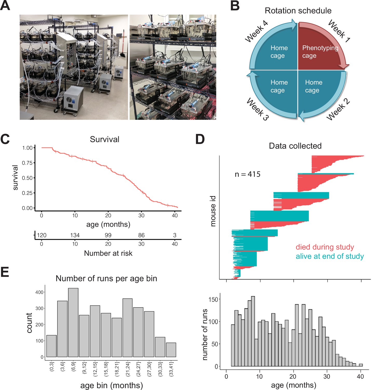
Study design.
(A) Pictures of automated cage phenotyping system. (B) Rotation schedule for each animal; each animal was monitored 1 week per month. (C) Survival of cohort. Vertical lines indicate censorship (still alive) at end of study. (D) Top: age range over which data was collected for each animal; each row represents one animal. Bottom: number of runs collected at each month of age. (E) Number of 7-day runs collected for each 3-month age bin. Most downstream analysis was performed using these bins.
Figure 1—figure supplement 1

Study design.
(A) Histogram of animal enrollment age. (B) Histogram of age at death for mice that died during study (n = 212, 51%). (C) Body mass distribution across entire dataset. (D) Body mass versus unadjusted energy expenditure. Each point represents one run. (E) Body mass versus mass-adjusted energy expenditure. Each point represents one run. (F) Pearson correlation coefficients for pairwise comparisons between all gas-derived measurements, before and after body mass correction. Analysis is based on the average value of each measurement for each run.
Figure 2 with 3 supplements
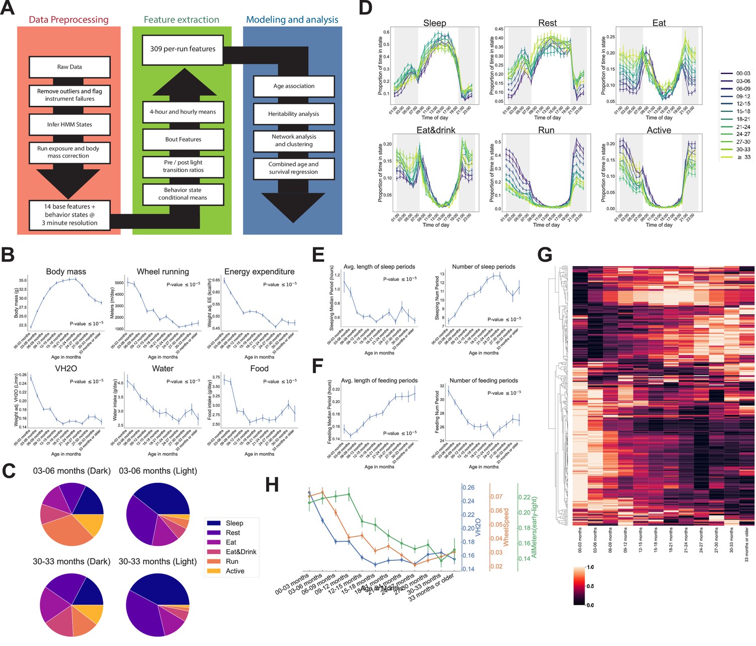
Automated phenotyping identifies physiological changes at each stage of life.
(A) Diagram of data processing pipeline. Three-min raw data from each run are fed through a quality control pipeline to remove data from broken and/or miscalibrated sensors. Data is then analyzed by a robust hidden Markov model (HMM) to assign each 3 min window to one of six states. Gas measurements are then adjusted for body mass. Data are then aggregated in a variety of ways for feature extraction: by time window (1 or 4 hr windows), by periods of behavior (e.g., number of sleeping periods), as a ratio of values from before and after a light transition (e.g., RQ pre-lights on/RQ post-lights on), and by state (e.g., VCO2 while running). Finally, data are used for modeling and analysis. (B) Effect of age on six of the base features of the phenotyping cages. Data were averaged for each run and then averaged across runs within each age bin. (C) Average percent time spent in each state for young (3–6 months) and old (30–33 months) animals, split by dark/light phase. (D) Average occupancy of each HMM state at each hour of the day. Timepoints represent the preceding hour, for example, the 7 pm timepoint includes data from 6 to 7 pm. (E) Effect of age on average duration and daily number of sleeping periods. (F) Effect of age on average duration and daily number of feeding periods. (G) Heatmap of aging trajectories. Rows are features (n = 309), columns are monthly age bins. Each feature was normalized and scaled across age bins from lowest value (0) to highest value (1). (H) Examples of four features that decrease with age, with different ages of onset. All error bars are SEM.
Figure 2—figure supplement 1
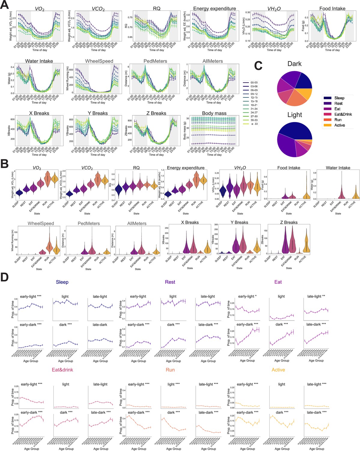
Automated phenotyping identifies robust physiological changes at each stage of life.
(A) Average hourly plots of the 14 base features of the phenotyping cage processing pipeline. Each run was grouped into 3-month age bins by the age of the mouse during that run. Timepoints represent the preceding hour, for example, the 7 pm timepoint includes data from 6 to 7 pm. (B) Base feature distribution in each of the hidden Markov model (HMM) states. Colors represent states. (C) Average percent of time spent in each state across entire cohort, split by dark/light phase. (D) Average occupancy of the six HMM states by age, separated in 4-hr time bins: early light (7–11 am), light (11 am–3 pm), late-light (3–7 pm), early-dark (7–11 pm), dark (11 pm–3 am), late-dark (3–7 am). Aging-associated corrected p-values indicated as *p < 0.05, **p < 0.01, ***p < 0.001.
Figure 2—figure supplement 2
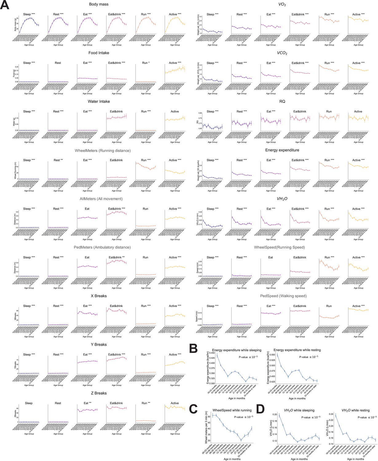
Effect of age on state-conditioned features.
(A) Effect of age on each of the 14 base features, plus WheelSpeed and PedSpeed, conditioned on hidden Markov model (HMM) state. Colors represent states. Aging-associated corrected p-values indicated as *p < 0.05, **p < 0.01, ***p < 0.001. (B) Expanded view of the effect of age on mass-adjusted energy expenditure (kcal/hr) during the lowest energy states: Sleep and Rest. (C) Expanded view of the effect of age on running speed, conditioned on animals being in the running state. (D) Expanded view of the effect of age on cage water vapor (VH2O) during the lowest energy states, Sleep and Rest. All error bars are SEM.
Figure 2—figure supplement 3
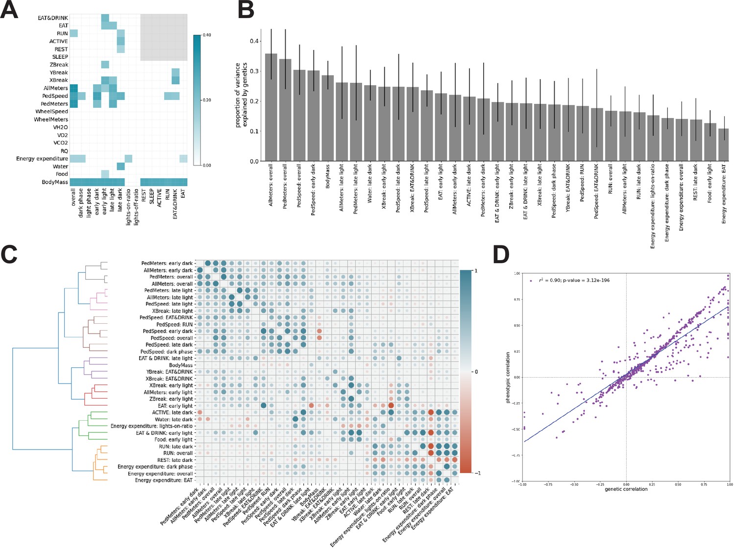
Genetic analysis of features.
(A) Heritability of features. Gray box indicates undefined features. (B) Forty-five features with significant nonzero heritability, sorted by descending heritability. (C) Pairwise genetic (lower triangle) and phenotypic (upper triangle) correlations, conditioned on age and cohort. Dendrogram represents hierarchical clustering of features using genetic correlation values. Each color represents a distinct cluster of features. (D) Scatterplot of phenotypic versus genetic correlation for each feature. Gray line depicts linear correlation (, ).
Figure 3 with 1 supplement

Quantifying relationships between physiological and behavioral features demonstrates a decline in resilience with age.
(A) Force-directed network diagram of all features across all runs. Nodes represent individual per-run features, edges reflect the regularized covariance between two features (effectively, the correlation between two features after accounting for all other features). Increased edge thickness indicates increased covariance. Colors represent predicted clusters. (B) Chord diagram of connectivity between clusters across all runs. Colors are as in (A). (C) Network connectivity at young and old age. Edges calculated for each age bin independently, with position of nodes held constant. (D) Effect of age on resilience, that is, the negative multivariate mutual information (MI) of the age-specific graphical model. A lower value indicates stronger connection between features and a lower diversity of states occupied by animals within that age bin. (E) Effect of age on inter-cluster resilience. Resilience calculated from age-specific sub-networks built from exemplar features, one from each cluster. (F) Effect of age on inter-cluster connectivity. Connectivity value represents the sum of all edges connecting cluster nodes to nodes in other clusters, that is, the same metric as in (B), plotted across age groups.
Figure 3—figure supplement 1
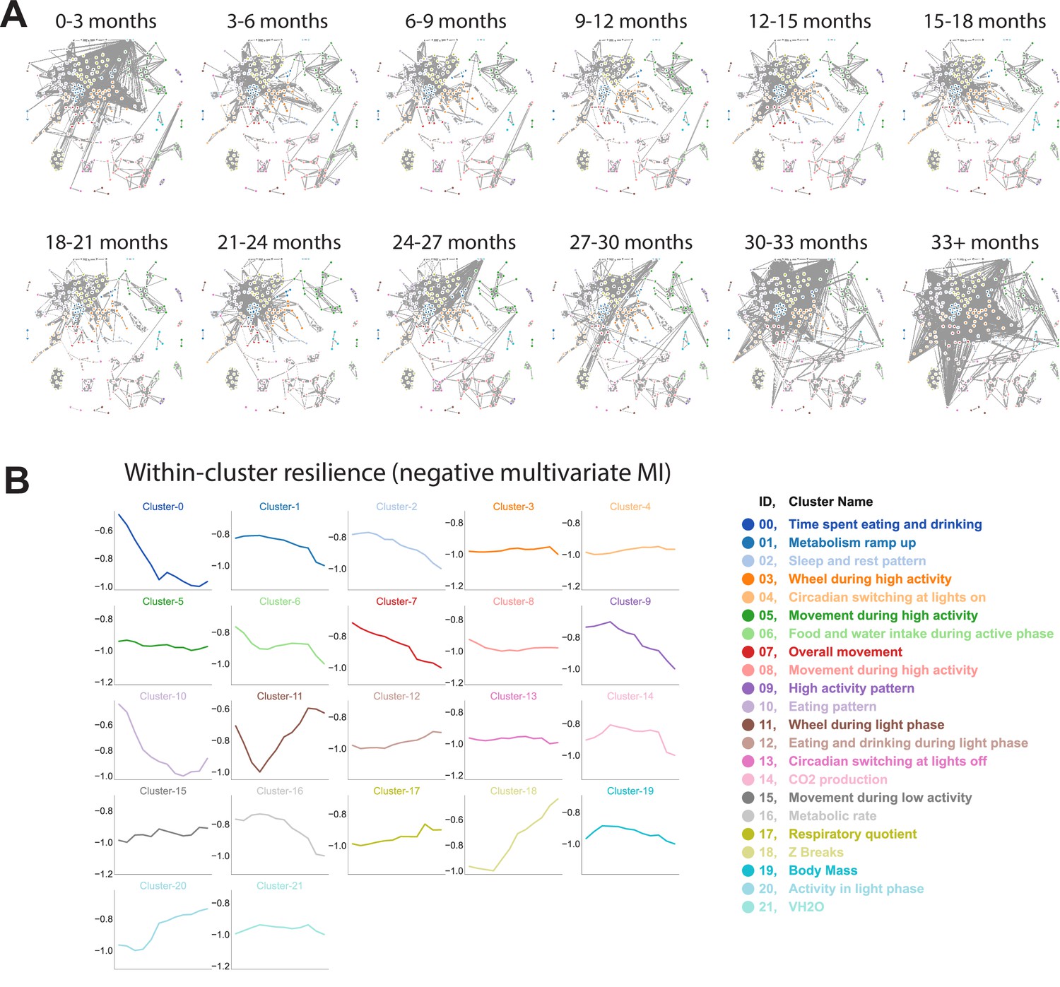
Physiological and behavioral network models.
(A) Network connectivity in each age bin. Edges calculated for each age bin independently, with position of nodes held constant. Increased edge thickness indicates increased covariance. Colors represent predicted clusters. (B) Effect of age on intra-cluster resilience for each cluster, determined using the connectivity between features within the same cluster.
Figure 4 with 1 supplement
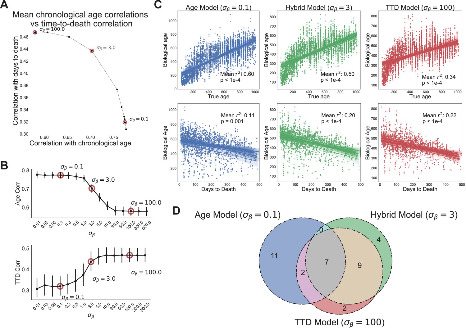
Age and time to death can be simultaneously predicted from physiological data.
(A) Correlation coefficient of CASPAR biological age predictions (test set) with time to death (y-axis) and chronological age (x-axis) for different values of , ranging from 0.1 to 100. Circled points represent values chosen for panels C and D. Correlation coefficients for each value of represents the average of 15 models trained against independent training/test data splits. (B) Correlation coefficient of biological age predictions (test set) with chronological age (top) and time to death (bottom) versus values. Error bars are SEM from the 15 models trained against independent training/test splits. (C) Scatterplots of predicted biological age versus chronological age (top) and time to death (bottom) for three different model classes (three different values of : 0.1, 3, 100). Points represent individual runs; all runs from each of the 15 independent test sets are shown. Lines represent linear regression for each of the 15 independent test sets. values are averages across the 15 test sets and p-values are of the median across the 15 test sets. (D) Venn diagram of the overlap between the top 20 most informative features for each of the three model classes noted above (age model, time to death model, hybrid model).
Figure 4—figure supplement 1
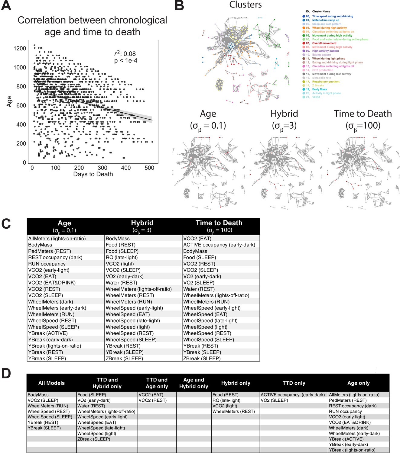
Age and time to death prediction.
(A) Correlation between chronological age (days) and time to death (days) across entire cohort. Each dot represents one run. (B) Top 20 most informative features for each Combined Aging and Survival Prediction of Aging Rate (CASPAR) model, annotated on overall network diagram. (C) Features shared by different models, as a reference for the Venn diagram in Figure 4D.
Additional files
-
Supplementary file 1
Univariate Kolmogorov-Smirnov test for each feature against age.
Rows are each of the 309 per-run features, columns are the KT coefficient, p-value with respect to age, Bonferroni-adjusted p-value, and a binary TRUE/FALSE significance column to indicate whether the adjusted p-value is less than 0.05. Percent of features with a significant age association is indicated on the right side of the table.
- https://cdn.elifesciences.org/articles/72664/elife-72664-supp1-v1.xlsx
-
Supplementary file 2
Features that comprise each of the clusters identified in Figure 3a.
Each column represents 1 of the 22 identified clusters. Row 1 indicates cluster number, row 2 indicates the qualitative name assigned to that cluster, and subsequent rows list the features that are included in that cluster.
- https://cdn.elifesciences.org/articles/72664/elife-72664-supp2-v1.xlsx
-
Transparent reporting form
- https://cdn.elifesciences.org/articles/72664/elife-72664-transrepform1-v1.docx
Download links
A two-part list of links to download the article, or parts of the article, in various formats.
Downloads (link to download the article as PDF)
Open citations (links to open the citations from this article in various online reference manager services)
Cite this article (links to download the citations from this article in formats compatible with various reference manager tools)
Automated, high-dimensional evaluation of physiological aging and resilience in outbred mice
eLife 11:e72664.
https://doi.org/10.7554/eLife.72664


