Figures and data in Minimal requirements for a neuron to coregulate many properties and the implications for ion channel correlations and robustness | eLife

Figures
Additional files

11 figures and 2 additional files

Figures

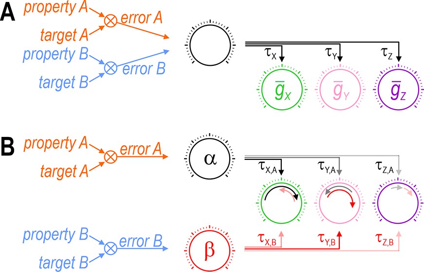
Figure 1

Download asset Open asset

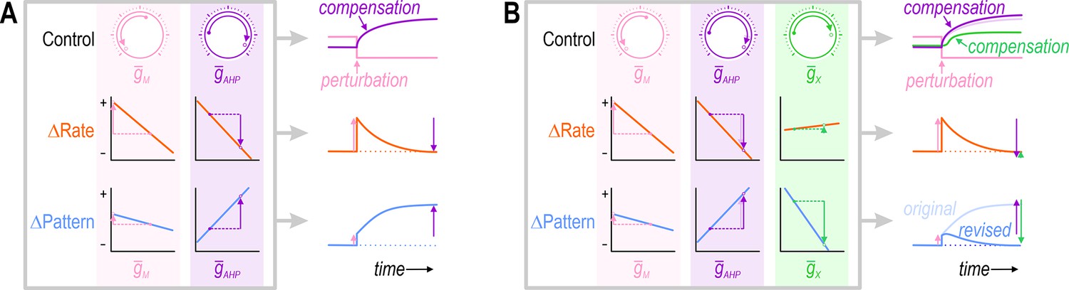
Simultaneous regulation of >1 property in a theoretical neuron.

(A) Challenge: If two ion channels, $g_{M}$ (pink) and $g_{A H P}$ (purple), both affect firing rate (orange), then the change in firing rate caused by perturbing $g_{M}$ can be offset by a compensatory change in $g_{A H P}$ . However, if $g_{M}$ and $g_{A H P}$ also affect firing pattern (blue), but not in exactly the same way, then the compensatory change in $g_{A H P}$ that restores firing rate to its target value may exacerbate rather than resolve the change in firing pattern. (B) Solution: Adjusting $g_{A H P}$ and at least one additional conductance, $g_{x}$ (green), that affects each property in a different way than $g_{A H P}$ , may enable firing rate and firing pattern to be regulated back to their target values. This suggests that the number of adjustable ion channels (‘dials’) relative to the number of regulated properties is important. Note that adjusting $g_{x}$ to restore the firing pattern necessitates a small extra increase in $g_{A H P}$ (compare pale and dark purple); in other words, conductances must be coadjusted.

Figure 2

Download asset Open asset

A compensatory change that restores firing rate disrupts firing pattern in a CA1 pyramidal neuron.

(A) Rasters show spiking in a single CA1 pyramidal neuron given the same noisy current injection (gray) on five trials under each of four conditions: baseline (blue), after blocking native I_M with 10 μM XE991 (black), and again after inserting virtual I_M (cyan) or virtual I_AHP (red) using dynamic clamp. See Methods for virtual conductance parameters. (B) Sample voltage traces under each condition. (C) Membrane potential differed across conditions (F_3,16 = 298.49, p < 0.001, one-way ANOVA); specifically, it was depolarized by blocking I_M (t = 18.71, p < 0.001, Tukey test) but that effect was reversed by inserting virtual I_M (t = 24.56, p < 0.001) or virtual I_AHP (t = 27.00, p < 0.001). (D) Spike amplitude also differed across conditions (F_3,16 = 154.04, p < 0.001); specifically, it was attenuated by blocking I_M (t = 20.23, p < 0.001) but that effect was reversed by inserting virtual I_M (t = 13.99, p < 0.001) or virtual I_AHP (t = 16.09, p < 0.001). (E) Firing rate also differed across conditions (F_3,16 = 177.61, p < 0.001); specifically, it was increased by blocking I_M (t = 18.38, p < 0.001) but that effect was reversed by inserting virtual I_M (t = 20.85, p < 0.001) or virtual I_AHP (t = 16.12, p < 0.001). (F) Regularity of spiking, reflected in the coefficient of variation of the interspike interval, also differed across conditions (F_3,16 = 188.23, p < 0.001), but whereas blocking I_M had a modest effect (t = 2.69, p = 0.048) and inserting virtual I_M had no effect (t = 0.39, p = 1.00), inserting virtual I_AHP had a large effect (t = 18.23, p < 0.001). Data are summarized as mean ± standard deviation (SD). Each data point represents a different trial from a single neuron. (G) Enlarged view of rasters to highlight spikes that occurred with native or virtual I_M but not with virtual I_AHP (blue shading) or vice versa (red shading) to illustrate the change in spike pattern caused by correcting the change in firing rate caused by blocking I_M with a compensatory change in I_AHP.

Figure 2—source data 1 Numerical values for experimental data plotted in Figure 2. Data include all spikes times (for panel A) as well as trial-averaged values of membrane potential, spike amplitude, firing rate, and coefficient of variation of the interspike interval (for panels C–F, respectively).: https://cdn.elifesciences.org/articles/72875/elife-72875-fig2-data1-v2.xlsx
Download elife-72875-fig2-data1-v2.xlsx

Figure 3 with 2 supplements

Download asset Open asset

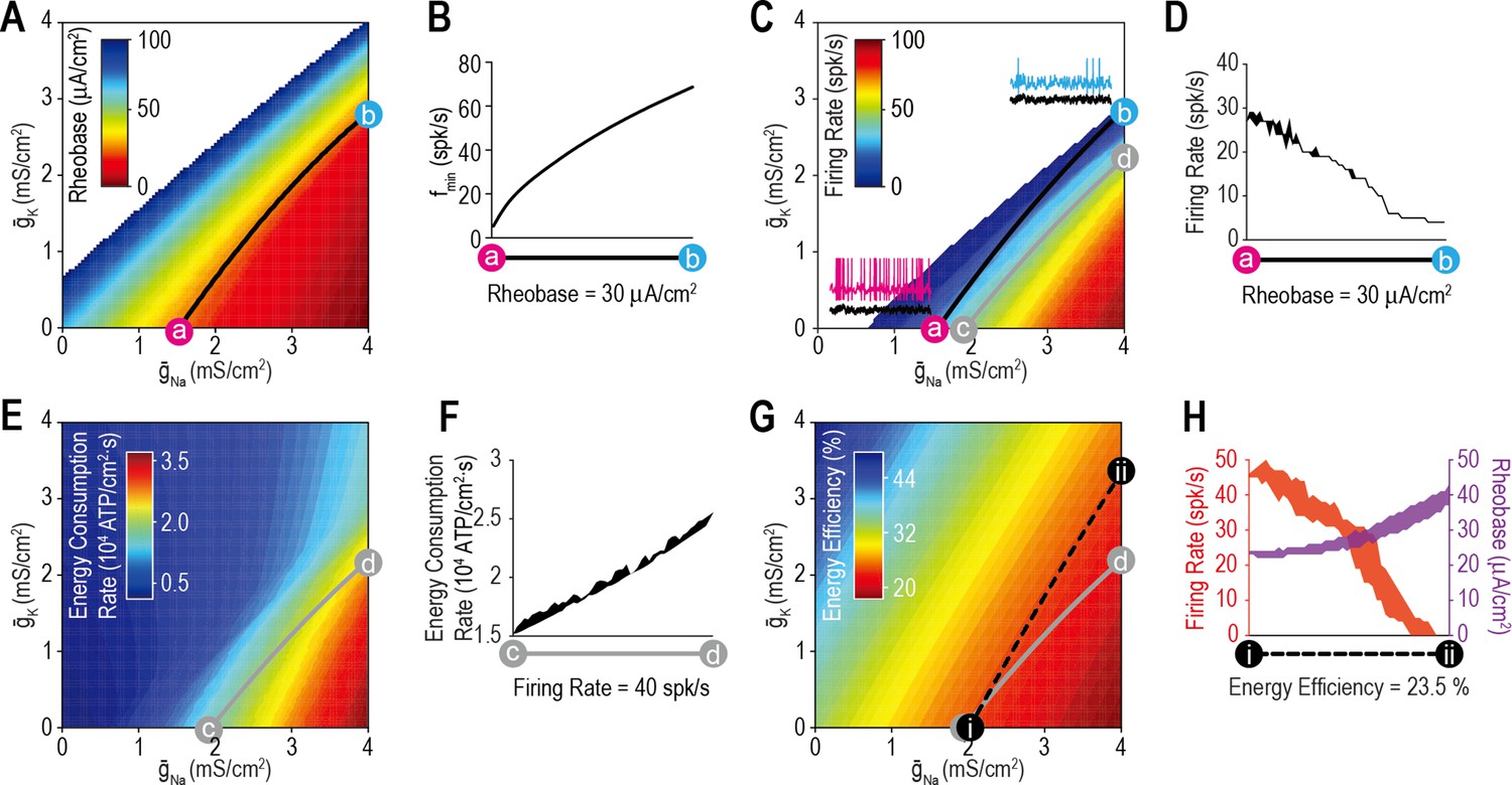
Most ion channel combinations producing the target value for one property produce inconsistent values for other properties.

(A) Color shows the minimum I_stim required to evoke repetitive spiking (rheobase) for different combinations of ${\bar{g}}_{N a}$ and ${\bar{g}}_{K}$ . Contour linking a and b highlights density combinations yielding a rheobase of 30 μA/cm². (B) Minimum sustainable firing rate (f_min) varied along the iso-rheobase contour (see Figure 3—figure supplement 1). (C) Color shows firing rate evoked by noisy I_stim (τ_stim = 5ms, σ_stim = 10 μA/cm², µ_stim = 40 μA/cm²) for different combinations of ${\bar{g}}_{N a}$ and ${\bar{g}}_{K}$ . Adding spike-dependent and -independent forms of adaptation ( ${\bar{g}}_{A H P}$ = 1.75 mS/cm² and ${\bar{g}}_{M}$ = 0.5 mS/cm²) broadened the dynamic range. Gray curve shows density combinations yielding a firing rate of 40 spk/s (i.e., an iso-firing rate contour; shown in red in Figures 4—6). Insets show sample responses to equivalent noisy stimulation. (D) Firing rate varied along the iso-rheobase contour from panel A. (E) Color shows energy consumption rate for different combinations of ${\bar{g}}_{N a}$ and ${\bar{g}}_{K}$ based on firing rates shown in panel C. Iso-firing rate contour c–d (gray line in panel C) does not align with energy contours. ATP consumed by the Na⁺/K⁺ pump was calculated from the total Na⁺ influx and K⁺ efflux determined from the corresponding currents. (F) Energy consumption rate varied along the iso-firing rate contour. (G) Color shows energy efficiency per spike for different combinations of ${\bar{g}}_{N a}$ and ${\bar{g}}_{K}$ . Energy efficiency was calculated as the capacitive minimum, CΔV, divided by total Na⁺ influx, where C is capacitance and ΔV is spike amplitude (see Figure 3—figure supplement 2). Density combinations along contour i–ii (dashed line) yield energy efficiency of 23.5% (shown in green in Figure 5). (H) Both rheobase and firing rate varied along the iso-energy efficiency contour.

Figure 3—figure supplement 1

Download asset Open asset

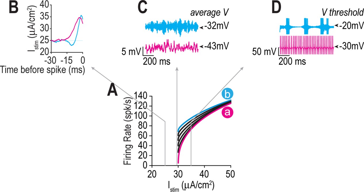
Ion channel combinations yielding equivalent rheobase produce different responses to noisy stimulation, reflecting fundamental differences in spike initiation dynamics and operating mode.

(A) Firing rate is shown as a function of I_stim for combination a (pink), b (cyan), and other values tested at 0.5 mS/cm² increments in ${\bar{g}}_{N a}$ (black) along the iso-rheobase contour a–b in Figure 3. Gray arrows point to responses to noisy stimulation modeled as an Ornstein–Uhlenbeck (OU) process with τ_stim = 5 ms and σ_stim = 5, 1, or 2 μA/cm² and μ_stim = 25, 29.5, or 35 μA/cm² for sub-, peri-, and suprathreshold conditions (panels B–D, respectively). (B) Spike-triggered averages (STAs) show that model a operates as an integrator with a longer integration time than model b, which operates as a coincidence detector. (C) Noise-induced membrane potential oscillations were slower for model a than for model b, consistent with differences in f_min, and average membrane potential differed by >10 mV. (D) Spike-dependent adaptation ( ${\bar{g}}_{A H P}$ = 2 mS/cm²) caused bursting in model b but not in model a. Voltage threshold also differed by 10 mV.

Figure 3—figure supplement 2

Download asset Open asset

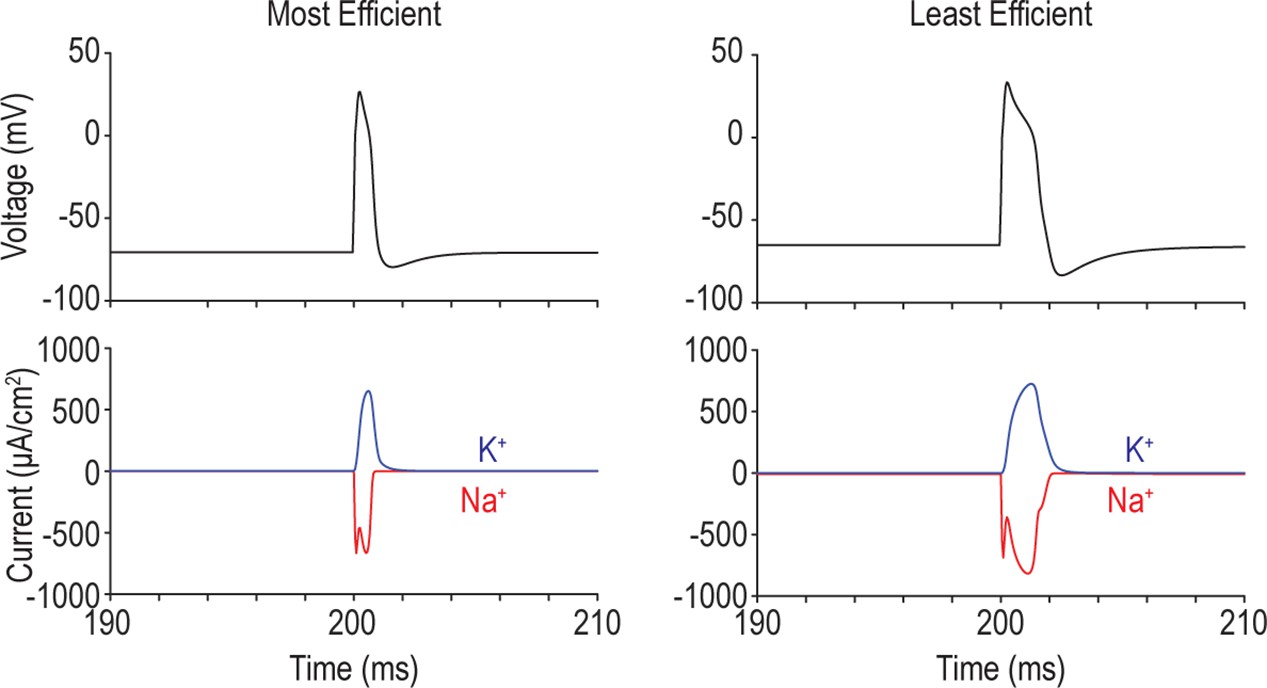
Overlap between Na⁺ and K⁺ currents dictates energy efficiency.

Voltage, total Na⁺ current, and total K ⁺ current during an action potential are shown for the most efficient (left) and least efficient (right) models. Simultaneous activation of Na⁺ and K ⁺ channels creates ‘waste’ current because Na⁺ influx and K ⁺ efflux cancel each other out. Overlap between Na⁺ and K ⁺ currents is larger in the model on the right, meaning more current is used relative to the theoretical minimum required to spike, which is calculated as CΔV, where C is the membrane capacitance and ΔV is the difference between the resting membrane potential and the spike peak.

Figure 4

Download asset Open asset

Ion channel changes mediating the same effect on firing rate can oppositely affect energy efficiency.

(A) Schematic shows how a difference in firing rate from its target value creates an error that is reduced by updating ${\bar{g}}_{N a}$ or ${\bar{g}}_{l e a k}$ . (B) Iso-firing rate contours for 40 spk/s are shown for different combinations of ${\bar{g}}_{N a}$ and ${\bar{g}}_{l e a k}$ with ${\bar{g}}_{K}$ at baseline (2 mS/cm², dashed red curve) and after ${\bar{g}}_{K}$ was ‘knocked out’ (0 mS/cm², solid red curve). When ${\bar{g}}_{K}$ was abruptly reduced, starting models (gray dots) spiked rapidly (~93 spk/s) before firing rate was regulated back to its target value by compensatory changes in either ${\bar{g}}_{N a}$ (pink) or ${\bar{g}}_{l e a k}$ (cyan). Models evolved in different directions and settled at different positions along the solid curve. (C) Trajectories show evolution of ${\bar{g}}_{N a}$ and ${\bar{g}}_{l e a k}$ . Trajectories are terminated once target firing rate is reached. Sample traces show responses before (gray) and immediately after (black) ${\bar{g}}_{K}$ was reduced, and again after compensatory changes in ${\bar{g}}_{N a}$ (pink) or ${\bar{g}}_{l e a k}$ (cyan). (D) Distributions of energy efficiency are shown before (gray) and after firing rate regulation via control of ${\bar{g}}_{N a}$ (pink) or ${\bar{g}}_{l e a k}$ (cyan).

Figure 5 with 1 supplement

Download asset Open asset

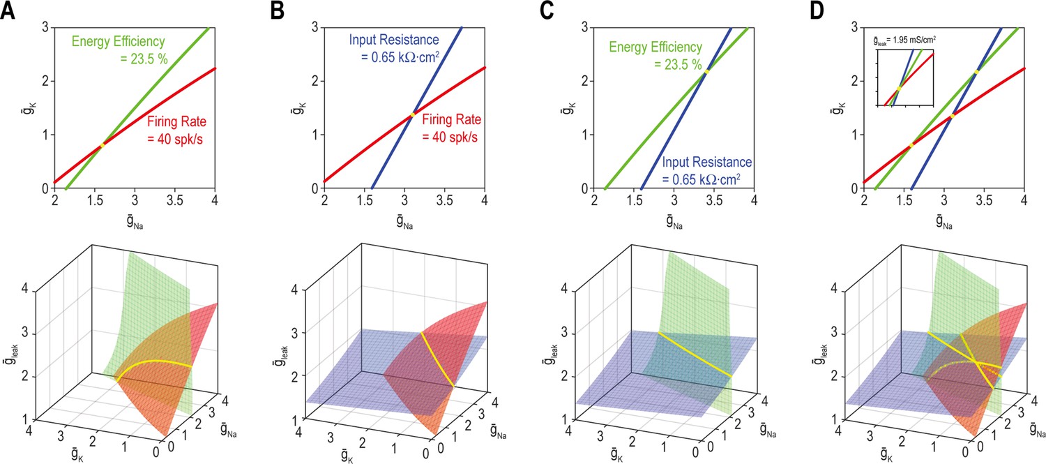
A degenerate solution for n properties requires at least n + 1 adjustable ion channels.

Curves in top panels depict single-output solutions sets based on control of ${\bar{g}}_{N a}$ and ${\bar{g}}_{K}$ (n_in = 2); ${\bar{g}}_{l e a k}$ = 2 mS/cm². Surfaces in bottom panels depict single-output solution sets based on control of ${\bar{g}}_{N a}$ , ${\bar{g}}_{K}$ , and ${\bar{g}}_{l e a k}$ (n_in = 3). Intersection (yellow) of single-output solutions at a point constitutes a unique multioutput solution, whereas intersection along a curve (or higher-dimensional manifold) constitutes a degenerate multioutput solution. (A) Curves for firing rate (40 spk/s) and energy efficiency (23.5%) intersect at a point whereas the corresponding surfaces intersect along a curve. Solutions for firing rate and input resistance (0.65 kΩ cm²) (B) and for energy efficiency and input resistance (C) follow the same pattern as in panel A. (D) For n_in = 2 (top), curves for firing rate, energy efficiency and input resistance do not intersect at a common point unless ${\bar{g}}_{l e a k}$ is reset to 1.95 mS/cm² (inset). For n_in = 3 (bottom), the three surfaces intersect at the same point as in the inset. See Figure 5—figure supplement 1 for the effects of tolerance on solution sets.

Figure 5—figure supplement 1

Download asset Open asset

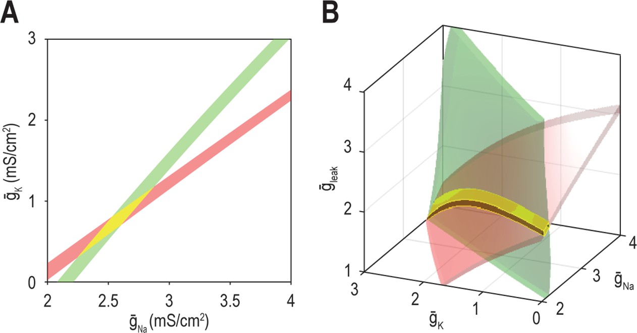
Increasing tolerance does not increase the dimensionality of multioutput solution sets the same way as increasing n_in.

(A) Curves for firing rate (40 spk/s) and energy efficiency (23.5%) expand into strips when tolerance (±3 spk/s and ±0.25%, respectively) is depicted. The strips intersect as a patch (yellow highlighting), unlike curves which intersect at a point (see Figure 5A, top). Note that 2D strips are limited to a 2D parameter space. The broad 2D surfaces that exist in 3D parameter space intersect along a long curve (see Figure 5A, bottom), unlike the small patch. (B) If ${\bar{g}}_{l e a k}$ is also controllable (n_in = 3), strips in 2D parameter space expand into shallow volumes in 3D parameter space. Those shallow volumes intersect along a narrow tube (yellow highlighting), which is unlike the broad surface formed by the intersection of deep volumes in 4D parameter space (not illustrated).

Figure 6

Download asset Open asset

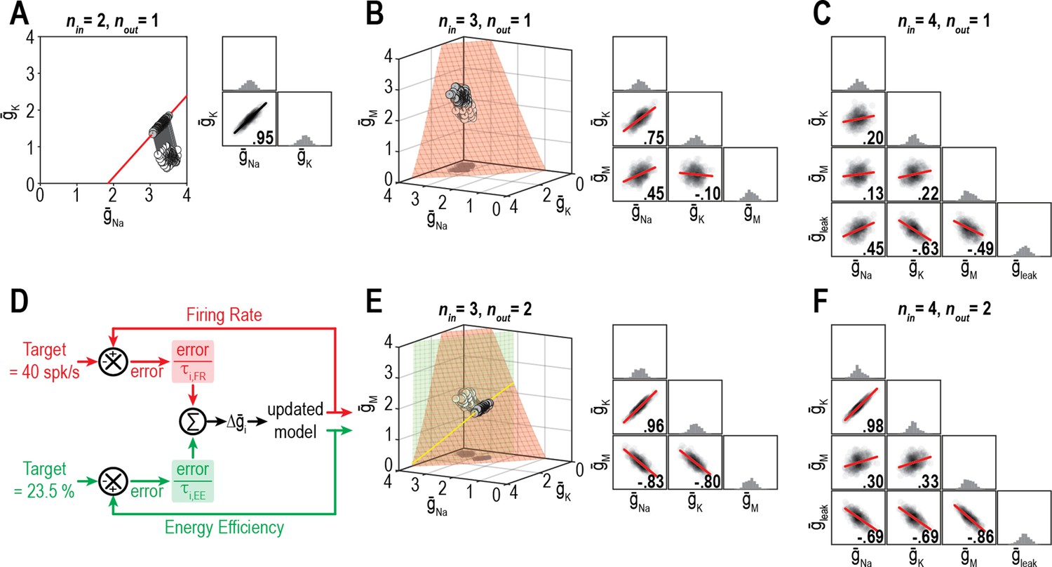
Dimensionality of solution space affects ion channel correlations.

(A) Starting from a normally distributed cluster of ${\bar{g}}_{N a}$ and ${\bar{g}}_{K}$ (white dots) yielding an average firing rate of 73 spk/s, ${\bar{g}}_{N a}$ and ${\bar{g}}_{K}$ (n_in = 2) were homeostatically adjusted to regulate firing rate (n_out = 1) to its target value of 40 spk/s. Gray lines show trajectories. Because solutions (gray dots) converge on a curve, the pairwise correlation between ${\bar{g}}_{N a}$ and ${\bar{g}}_{K}$ is predictably strong. Scatter plots show solutions centered on the mean and normalized by the standard deviation (z-scores). Correlation coefficient (R) is shown in the bottom right corner of each scatter plot. (B) Same as panel A (n_out = 1) but via control of ${\bar{g}}_{N a}$ , ${\bar{g}}_{K}$ , and ${\bar{g}}_{M}$ (n_in = 3). Homeostatically found solutions converge on a surface and ion channel correlations are thus weaker. (C) If ${\bar{g}}_{l e a k}$ is also controlled (n_in = 4), solutions converge on a hard-to-visualize volume (not shown) and pairwise correlations are further weakened. (D) Schematic shows how errors for two regulated properties are combined: the error for each property is calculated separately and is scaled by its respective control rate τ to calculate updates, and all updates for a given ion channel (i.e., originating from each error signal) are summed. (E) Same as panel B (n_in = 3), but for regulation of firing rate and energy efficiency (n_out = 2). Homeostatically found solutions once again converge on a curve (yellow), which now corresponds to the intersection of two surfaces; ion channel correlations are thus strong, like in panel A. (F) If n_in is increased to four while n_out remains at 2, solutions converge on a surface (not shown) and ion channel correlations weaken.

Figure 7

Download asset Open asset

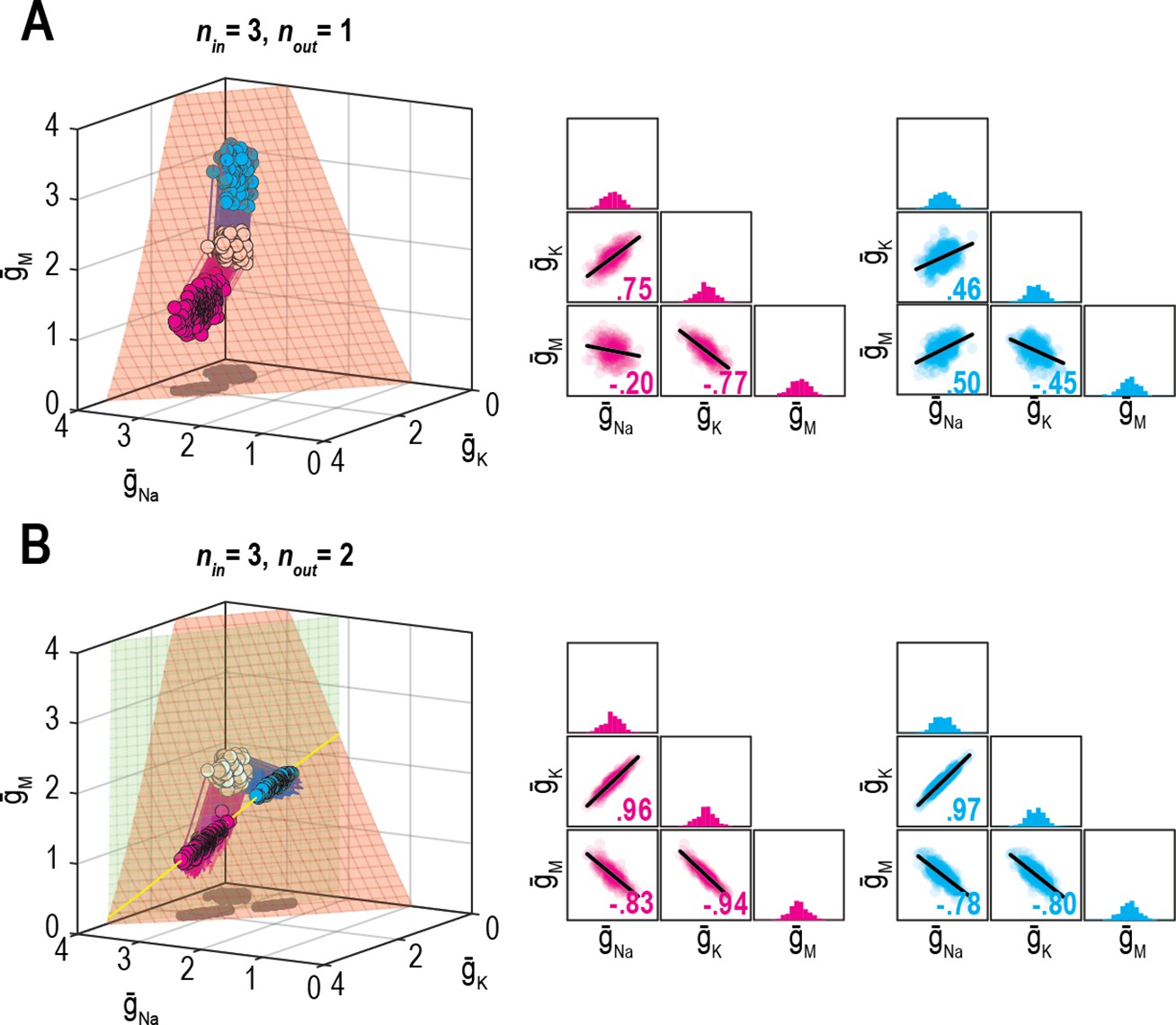
Effect of relative regulation rates on ion channel correlations depends on the dimensionality of solution space.

(A) Homeostatic regulation of firing rate via control of ${\bar{g}}_{N a}$ , ${\bar{g}}_{K}$ , and ${\bar{g}}_{M}$ . Same as Figure 6B, but for two new sets of regulation rates (see Supplementary file 1). Solutions found for each set of rates (pink and cyan) approached the surface from different angles and converged on the surface with different patterns, thus producing distinct ion channel correlations, consistent with O’Leary et al., 2013. (B) Same as panel A (n_in = 3), but for homeostatic regulation of firing rate and energy efficiency (n_out = 2). Solutions converge on a curve (yellow), giving rise to virtually identical ion channel correlations regardless of regulation rates.

Figure 8 with 1 supplement

Download asset Open asset

Noise can affect ion channel correlations depending on the dimensionality of solution space.

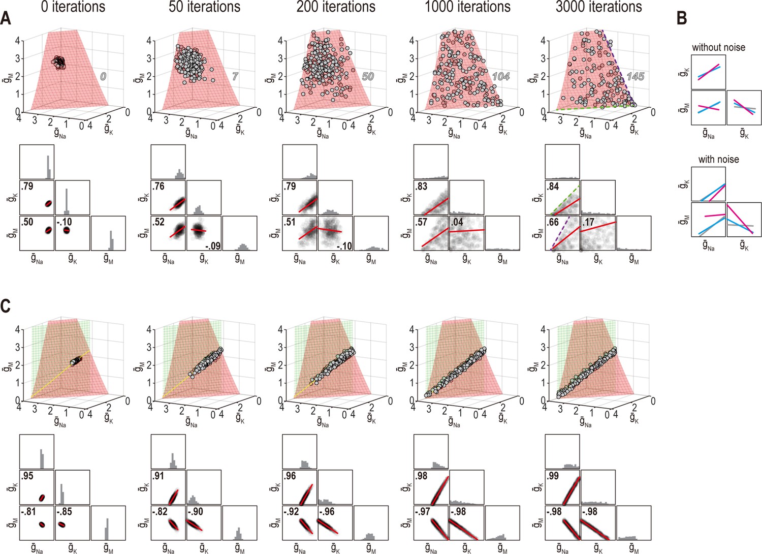
(A) Starting from solution sets in Figure 6B, ${\bar{g}}_{N a}$ , ${\bar{g}}_{K}$ , and ${\bar{g}}_{M}$ had noise added to them and were then updated by homeostatic regulation (using regulation rates from Figure 6) to correct the noise-induced disruption of firing rate. Conductance density combinations are depicted before and after 50, 200, 1000, or 3000 noise-update iterations (left to right). Noise caused solutions to spread across the surface (top). Some solutions (number in italics) drifted beyond the illustrated region but this is prevented by imposing an upper bound (Figure 8—figure supplement 1A). Ion channel correlations reflect the available solution space; for example, changes in ${\bar{g}}_{N a}$ and ${\bar{g}}_{K}$ are limited by ${\bar{g}}_{M}$ remaining positive (dashed green line), while changes in ${\bar{g}}_{N a}$ and ${\bar{g}}_{M}$ are limited by ${\bar{g}}_{K}$ remaining positive (dashed purple line). How solutions distribute within that space depends on regulation rates, and also affects correlations (Figure 8—figure supplement 1B, C). Conductance density distributions and pairwise correlations (bottom) were not centered on the mean or normalized by standard deviation (unlike in other figures) in order to visualize how distributions evolve over iterations. (B) Comparison of regression lines from Figure 6 (gray) and 7 (pink, cyan) without noise (top) and with noise (bottom). Correlations are affected by regulation rates in both conditions, but not in the same way. (C) Same as panel A but for regulation of firing rate and energy efficiency. Solutions spread along the intersection of the two surfaces, but the spread is bounded by one or another conductance density reaching 0 mS/cm². Correlations slightly increase under noisy conditions (compare with Figure 6).

Figure 8—figure supplement 1

Download asset Open asset

Correlations depend on the solution manifold’s shape and how solutions distribute across it.

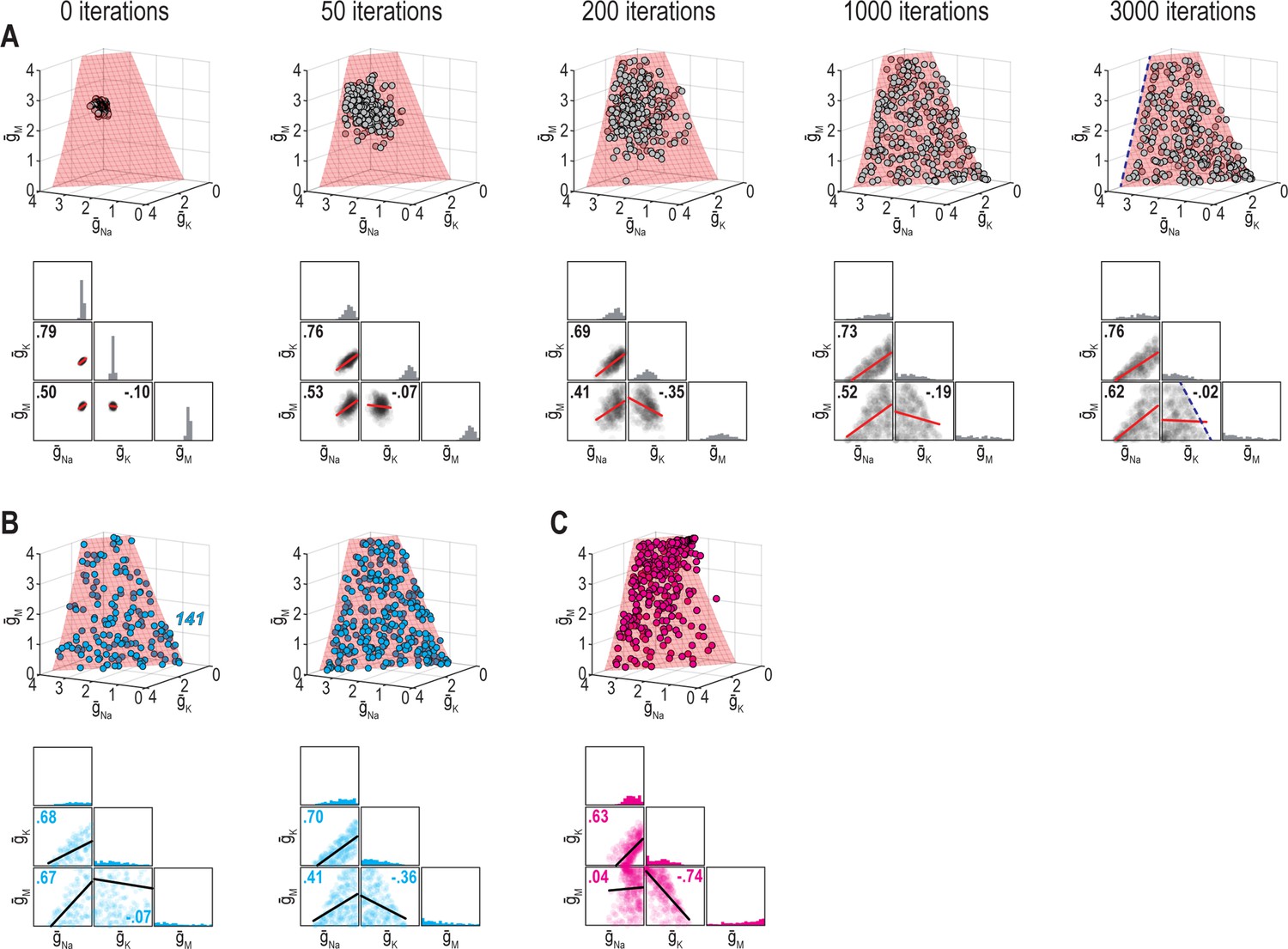
(A) Same conditions as in Figure 8A but with conductance densities restricted from increasing above 4 mS/cm², thus preventing solutions from drifting beyond the illustrated region. An upper bound on conductance densities almost certainly exist since transcript and protein levels reflect an equilibrium of production and degradation, where rate-limiting production steps saturate (Schwanhäusser et al., 2011). Imposing an upper bound further constrains the spread of solutions and shapes correlations; for example, changes in ${\bar{g}}_{K}$ and ${\bar{g}}_{M}$ are constrained by ${\bar{g}}_{M}$ remaining below 4 mS/cm² (dashed blue line). (B) Effect of noise after 3,000 iterations without (left) and with (right) an upper bound, using cyan regulation rates from Figure 7. (C) Same as right panel in B but using pink regulation rates from Figure 7. Noise causes solutions to spread across the manifold but solutions can drift preferentially in a certain direction depending on regulation rates; for example, solutions drift upward and yield high values of ${\bar{g}}_{M}$ for pink regulation rates, whereas the opposite occurred for the other regulation rates. The distribution of points affects correlations (see Figure 8B).

Figure 9

Download asset Open asset

Low-dimensional solutions can be hard for homeostatic regulation to ‘find’.

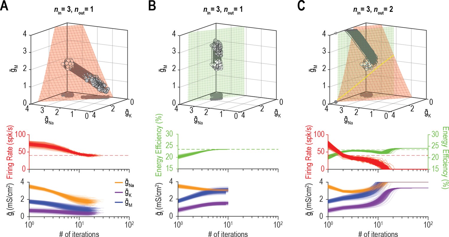
(A) Homeostatic regulation of firing rate (n_out = 1) via control of ${\bar{g}}_{N a}$ , ${\bar{g}}_{K}$ , and ${\bar{g}}_{M}$ (n_in = 3), like in Figures 6B and 7A but using a different set of regulation rates (see Supplementary file 1). Solutions converged onto the iso-firing rate surface (top panel) and firing rate was regulated to its target value in <30 iterations (bottom panel). (B) Same as A (n_in = 3) but for homeostatic regulation of energy efficiency (n_out = 1). Solutions converged on the iso-energy efficiency surface (top panel) and energy efficiency was regulated to its target value in ~10 iterations (bottom panel). (C) Homeostatic regulation of firing rate and energy efficiency (n_out = 2) via control of the same ion channels (n_in = 3) using the same relative rates and initial values as in panels A and B. Neither firing rate (red trajectories) nor energy efficiency (green trajectories) reached its target value. Conductance densities were capped at 4 mS/cm² but this does not account for trajectories not reaching their target. Noise was not included in these simulations.

Figure 10

Download asset Open asset

The outcome of homeostatic regulation depends on if and how single-output solution sets intersect.

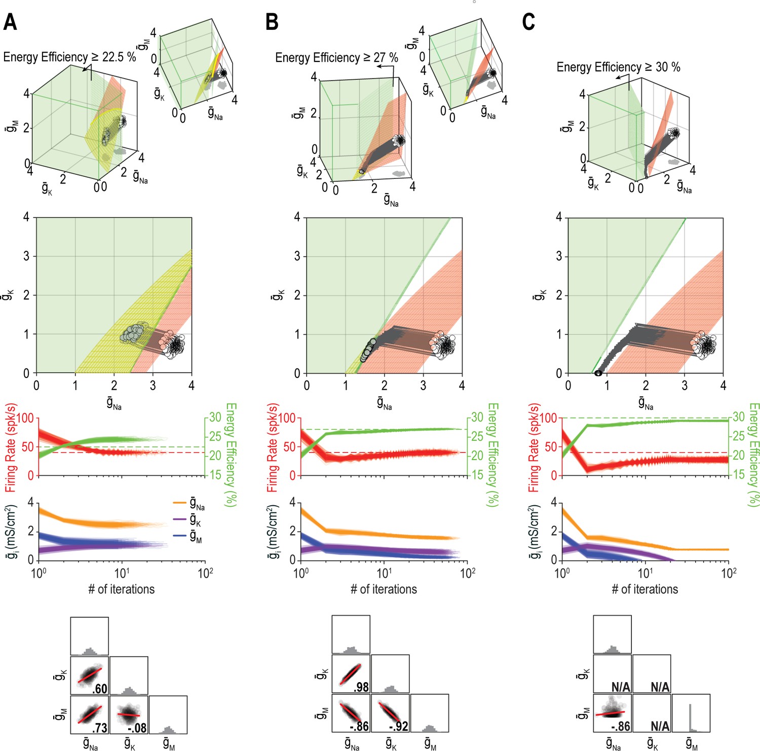
Homeostatic regulation of firing rate and energy efficiency (n_out = 2) via control of ${\bar{g}}_{N a}$ , ${\bar{g}}_{K}$ , and ${\bar{g}}_{M}$ (n_in = 3). For these simulations, energy efficiency was maintained above a lower bound rather than being regulated to a specific target value; accordingly, the single-output solution set for energy efficiency corresponds to a volume (green) rather than a surface. (A) For energy efficiency ≥22%, homeostatically determined solutions converge on the iso-firing rate surface (red) in a region sitting within the green volume (top panel). The rate of convergence and resulting ion channel correlations are shown in the middle and bottom panels, respectively. (B) For energy efficiency ≥27%, solutions initially converge on the red surface in a region outside the green volume, but trajectories then bend and proceed across the red surface until that surface reaches the green volume. Because solutions converge on a curve, ion channel correlations are stronger than in A, where solutions distributed across a surface. (C) For energy efficiency ≥30%, the red surface and green volume do not intersect. Consequently, solutions settle between the two single-output solution sets (top panel) without either property reaching its target (middle panel). The outcome represents the balance achieved by the opposing pull of control mechanisms regulating different properties, and depends entirely on ${\bar{g}}_{N a}$ since ${\bar{g}}_{K}$ and ${\bar{g}}_{M}$ cannot become negative (bottom panel). Noise was not included in these simulations.

Figure 11

Download asset Open asset

Each error signal must be able to coadjust channels with different ratios.

Cartoons depict regulation of two properties (A and B) via control of three ion channels (X, Y, and Z). Channel levels are homeostatically adjusted to minimize the difference (error) between each property and its target value. The error signal divided by each channel’s regulation time constant (τ) dictates the magnitude of the change in that channel (represented by length of curved arrows in panel B). (A) The set of regulation time constants define a ‘master regulator’ (black dial) that coadjusts ion channels according to a certain ratio. Convergence of error signals at or before the master regulator limits how ion channels are coadjusted. (B) An additional master regulator (red dial) is needed to enable error B to coadjust channels with a different ratio than error A. Conditions like in panel B were required for all coregulation simulations (see Figure 6C). Different coadjustment ratios are required to regulate each property because of the different way each ion channel affects each property (see Figure 1). Note that master regulators may be more distributed than depicted here, with each regulation time constant τ_i,j likely reflecting the net effect of regulating multiple (transcriptional, translational, etc.) processes. The positive molecular regulatory network proposed by Franci et al., 2020 involves additional feedback mechanisms not easily depicted in this sort of cartoon.

Additional files

Supplementary file 1 Initial conductance densities and regulation time constants used for simulations. When a conductance is not regulated, its density was fixed at the average.: https://cdn.elifesciences.org/articles/72875/elife-72875-supp1-v2.xlsx
Download elife-72875-supp1-v2.xlsx
Transparent reporting form: https://cdn.elifesciences.org/articles/72875/elife-72875-transrepform1-v2.docx
Download elife-72875-transrepform1-v2.docx

Download links

A two-part list of links to download the article, or parts of the article, in various formats.

Downloads (link to download the article as PDF)

Open citations (links to open the citations from this article in various online reference manager services)

Mendeley

Cite this article (links to download the citations from this article in formats compatible with various reference manager tools)

Jane Yang
Husain Shakil
Stéphanie Ratté
Steven A Prescott

(2022)

Minimal requirements for a neuron to coregulate many properties and the implications for ion channel correlations and robustness

eLife 11:e72875.

https://doi.org/10.7554/eLife.72875

Sign up for email alerts

Privacy notice