The Digital Brain Bank, an open access platform for post-mortem imaging datasets
- Wellcome Centre for Integrative Neuroimaging, FMRIB, Nuffield Department of Clinical Neurosciences, University of Oxford, United Kingdom
- Division of Clinical Neurology, Nuffield Department of Clinical Neurosciences, University of Oxford, United Kingdom
- Psychology Department, Emory University, United States
- Centre for Zoo and Wild Animal Health, Copenhagen Zoo, Denmark
- Department of Radiology, University of Chicago, United States
- Department of Complex Trait Genetics, Centre for Neurogenomics and Cognitive Research, Amsterdam Neuroscience, Vrije Universiteit Amsterdam, Netherlands
- Department of Child Psychiatry, Amsterdam Neuroscience, Amsterdam UMC, Vrije Universiteit Amsterdam, Netherlands
- Medical Research Council Oxford Institute for Radiation Oncology, University of Oxford, United Kingdom
- School of Anatomical Sciences, Faculty of Health Sciences, University of the Witwatersrand, South Africa
- Wellcome Centre for Integrative Neuroimaging, Department of Experimental Psychology, University of Oxford, United Kingdom
- Stem Cell and Brain Research Institute, Université Lyon 1, INSERM, France
- Donders Institute for Brain, Cognition and Behaviour, Radboud University Nijmegen, Netherlands
Figures
Figure 1
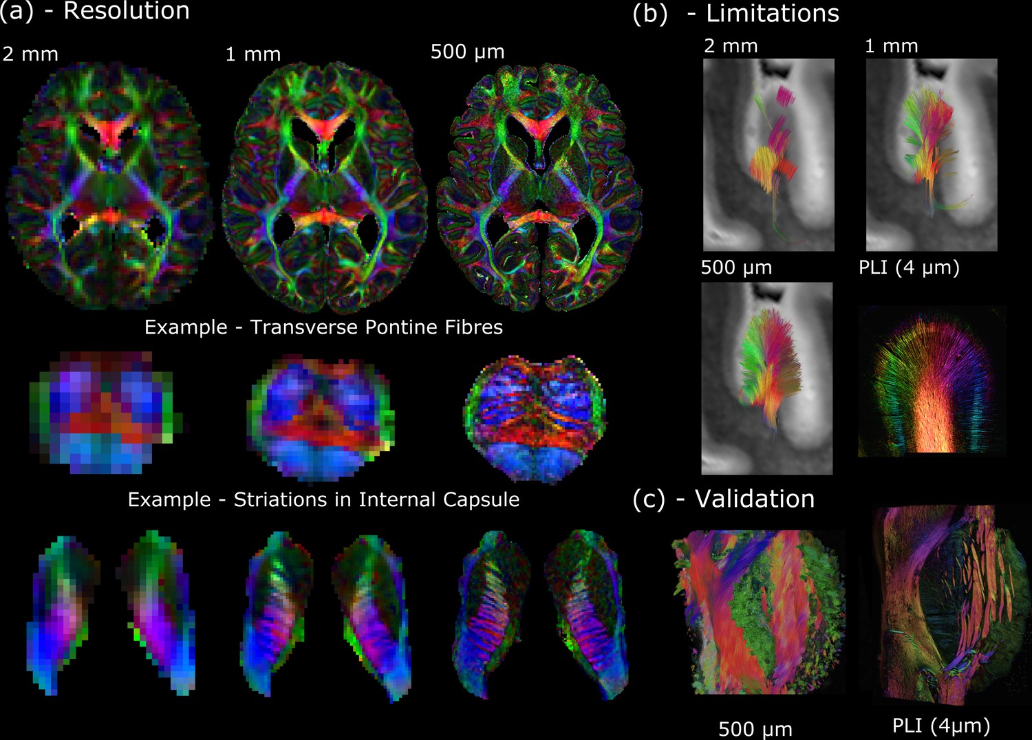
The Digital Anatomist.
(a) Whole-brain diffusion MRI data available in the Human High-Resolution Diffusion MRI-PLI dataset reveals the wealth of information provided at increased spatial scales, one of the key aims of the Digital Anatomist. Here, the 500 μm dataset uncovers the information hidden at lower spatial resolutions, for example, visualizing the interdigitating transverse pontine fibers with the corticospinal tract or striations through the internal capsule. (b) Similarly, datasets across multiple spatial scales can inform us of the limitations at reduced imaging resolutions. Here, gyral tractography (occipital lobe) reveals an overall pattern of fibers turning into the gyral bank at 0.5 mm. At 1 mm, an underestimation of connectivity at the gyral banks is observed, known as the ‘gyral bias’ (Cottaar et al., 2021; Schilling et al., 2018). At 2 mm, tractography bears little resemblance to the expected architecture. Multimodal comparisons enable us to validate our findings, with complementary polarised light imaging (PLI) data at over 2 orders of magnitude increase in resolution (125×) revealing a similar pattern of gyral connectivity, and (c) excellent visual agreement with tractography across the pons. (a) displays diffusion tensor principal diffusion direction maps (modulated by fractional anisotropy).
Figure 2
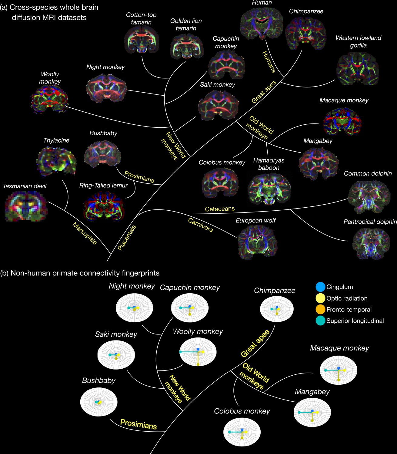
The Digital Brain Zoo.
(a) The first release of the Digital Brain Zoo provides whole-brain MRI datasets spanning multiple species and taxonomic ranks. Notably, we provide whole-brain diffusion MRI datasets from 14 nonhuman primate species, with samples selected for their high quality and to ensure sampling of all major branches of the primate evolutionary tree (Prosimian, New World monkey, Old World monkey, and Great Ape). (b) compares the relative volume of four tracts derived from nine nonhuman primate post-mortem datasets provided in the Digital Brain Zoo (Bryant et al., 2021), where increased distance from the centre corresponds to an increased volume.
Figure 3

The Digital Pathologist.
One of the key aims of the Digital Pathologist is the examination of neuropathological spread in neurological disease. The Human ALS MRI-Histology dataset (a) facilitates these investigations, combining whole-brain multimodal MRI and histology (selected brain regions) in a cohort of 12 ALS and 3 control brains. (b) Displays the reconstruction of five white matter pathways associated with different ALS stages in a single post-mortem brain (Kassubek et al., 2014). Comparisons between ALS and control brains over the corpus callosum of the cohort (c) reveals changes in fractional anisotropy (FA, normalized to Par/Temp/Occ lobe), with biggest changes associated with motor and prefrontal regions (Hofer and Frahm, 2006) (*=p<0.05; **=p<0.05 following multiple comparison correction) (full details of the corpus callosum analysis provided in Appendix 2). This reflects the anticipated changes in ALS with brain regions associated with motor function, in good agreement with a previous study (Chapman et al., 2014), which identified the greatest FA difference between ALS and controls in these regions. Accurate MRI-histology coregistrations facilitate cross-modality comparisons, and (d) displays an example of MRI-histology coregistration over the visual cortex of a single ALS brain achieved using the Tensor Image Registration Library (TIRL) (Huszar et al., 2019). V1=principal diffusion direction, FA=fractional anisotropy, MD=mean diffusivity, D⊥=radial diffusivity, MO=mode from diffusion tensor output, Dyad1=principal dyad orientation, f1=principal fiber fraction and D=diffusivity from Ball and Two-Stick output, swMRI=susceptibility-weighted MRI, χ=magnetic susceptibility. Details of stain contrasts in (b) and (d) are provided in Table 1. ALS, amyotrophic lateral sclerosis; MRI, magnetic resonance imaging.
Appendix 3—figure 1
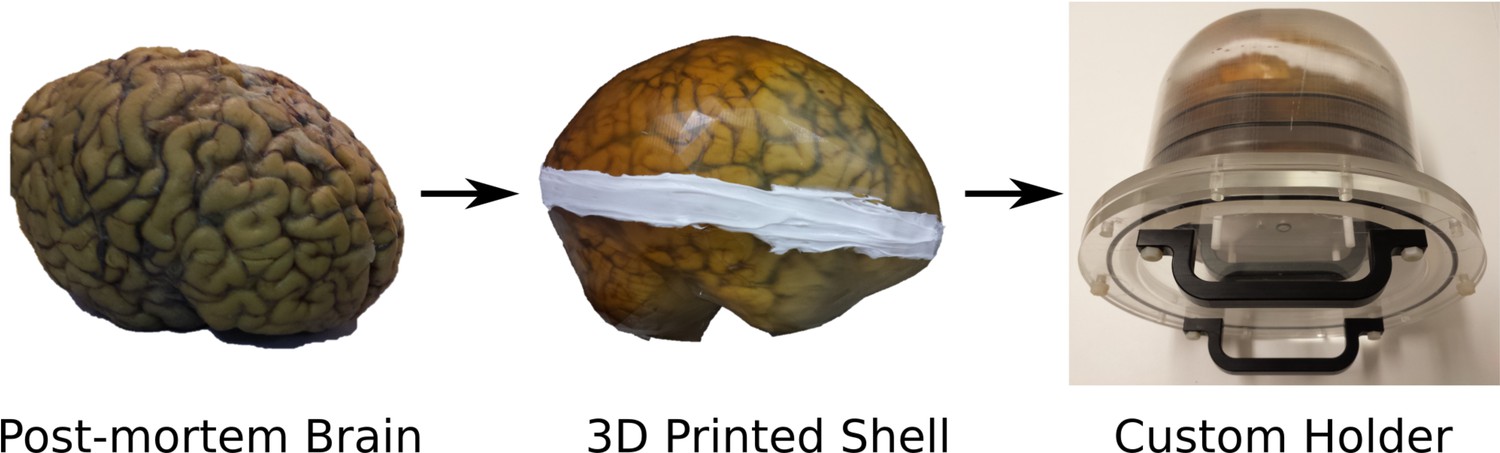
Post-mortem human brain holder.
The brain holder ensures consistent placement during scanning. Here, the custom holder tightly seals the brain in place, whilst the 3D printed shell (provided by Dr Alard Roebroeck, Maastricht University) prevents pressure on the brain. The holder is designed with a spherical cavity to maximize field homogeneity. For further information on our scanning procedure for human post-mortem brains, see Wang et al., 2020.
Appendix 3—figure 2
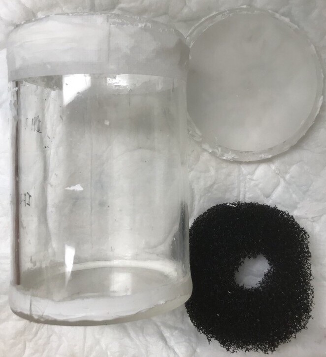
Post-mortem cylindrical brain holder.
The brain holder used for scanning large nonhuman brains which fit inside the 28 channel QED knee coil. This consisted of a cylindrical container, with plastic gauze (black) used to secure samples during the acquisition.
Appendix 4—figure 1
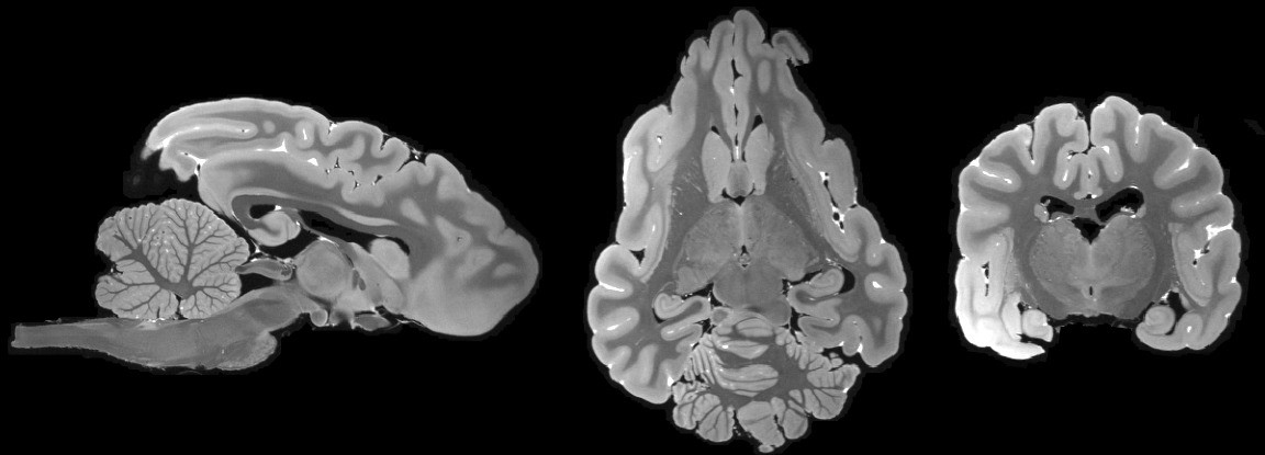
Structural MRI.
Example structural MRI dataset acquired using a bSSFP sequence in the European wolf (Canis lupus) at a resolution of 220 μm (isotropic). bSSFP Structural MRI datasets display excellent gray-white matter contrast, facilitating the delineation of fine tissue structures and integration with processing pipelines for surface reconstruction. Contrast in bSSFP datasets is reversed compared to conventional T1-weighted structural MRI scans (gray matter appears bright, and white matter appears dark), which must be accounted for in any analysis pipeline.
Tables
Table 1
Description of all datasets provided in the first release to the Digital Brain Bank.
All Structural MRI datasets in the first release were acquired using a balanced SSFP (bSSFP) or T2-weighted sequence, which yields strong gray-white matter contrast in formalin-fixed post-mortem tissue. Diffusion MRI datasets were acquired using a combination of diffusion-weighted steady-state free precession (DW-SSFP) and diffusion-weighted spin-echo (DW-SE) sequences. Full details of the motivation behind the choice of sequences and available contrasts are described in the Discussion. †T2* and magnetic susceptibility maps are currently available in 9 out of 12 ALS brains and all control brains. The remaining datasets were either lost during scanner export, or are of insufficient data quality for public release.
| Category | Name | Contents: MRI | Resolution (MRI) | Contents: Microscopy | Relevant publications |
|---|---|---|---|---|---|
| Digital Anatomist | Human High-Resolution Diffusion MRI-PLI | Whole-brain diffusion MRI, structural MRI, quantitative T1 and T2 maps: – Control human brain: 1× | Diffusion MRI: (500 μm, 1 and 2 mm iso.) Structural MRI: 312.5×312.5×500 μm3 T1 map: (0.75×0.75×1.6 mm3) T2 map: (0.75×0.75×1.6 mm3) | Polarised light imaging (4 μm in-plane) in the anterior commissure, corpus callosum, pons, thalamus, and visual cortex (same brain) | Dataset described in this publication (Methodology in Appendix 1), Diffusion MRI processing described in Tendler et al., 2020b, T2 mapping described in Tendler et al., 2021 |
| Digital Anatomist | Human Callosum MRI-PLI-Histology | Corpus callosum diffusion MRI: – Excised control human corpus callosum samples: 3× | Diffusion MRI: (400 μm iso.) | Polarised light imaging (4 μm in-plane), bright-field microscopy images of immunohistochemistry stains (0.25 μm in-plane) for PLP (myelin) and GFAP (astrocyte) (same human corpus callosum samples) | Mollink et al., 2017 |
Whole-brain diffusion MRI and structural MRI (available in brains marked with a *):
| Diffusion MRI: 300 μm iso.: Bushbaby, Cotton-Top tamarin & Golden Lion Tamarin 400 μm iso: Night monkey 500 μm iso: Ring-tailed lemur and Saki monkey 600 μm iso: Capuchin monkey, Chimpanzee, Colobus monkey, Hamadryas baboon, Macaque monkey, Mangabey, Western Lowland Gorilla and Woolly Monkey Structural MRI 200 μm iso: Western Lowland Gorilla 220 μm iso: Hamadryas Baboon 0.22×0.22×0.19 mm3: 1× Chimpanzee 0.375×0.375×0.40 mm3: 1× Chimpanzee | None | 1× Western Lowland gorilla and 1× Chimpanzee described in Roumazeilles et al., 2020, 3× Macaque monkey and 3× Ring-Tailed Lemur described in Roumazeilles et al., 2021. Hamadryas baboon, Cotton-Top tamarin and Golden Lion tamarin datasets described in this publication (Methodology in Appendix 1). All other datasets described in Bryant et al., 2021 | ||
| Digital Brain Zoo | Marsupials | Whole-brain diffusion MRI and structural MRI:
| Diffusion MRI: 1 mm iso: 1× Tasmanian devil 1.5 mm iso: 1× Tasmanian devil 1.1 mm iso: 1× Thylacine 1.0×1.1×0.8 mm3: 1× Thylacine Structural MRI 330 μm iso: 1× Tasmanian devil and 1× Thylacine 330×330×300 μm3: 1× Tasmanian devil 500 μm iso: 1× Thylacine | None | Berns and Ashwell, 2017 |
| Digital Brain Zoo | Cetaceans | Whole-brain diffusion MRI and structural MRI
| Diffusion MRI: (1.3 mm iso.) Structural MRI: (640×640×500 μm3) | None | Berns et al., 2015 |
| Digital Brain Zoo | Carnivora | Whole-brain diffusion MRI and structural MRI: – European wolf (Canis lupus): 1× | Diffusion MRI: (600 μm iso.) Structural MRI: (220 μm iso.) | None | Dataset described in this publication (Methodology in Appendix 1) |
| Digital Pathologist | Human ALS MRI-Histology | Whole-brain diffusion MRI, structural MRI, quantitative T1, T2, and T2* maps, magnetic susceptibility maps (selected brains†):
| Diffusion MRI: (850 μm iso.) Structural MRI: (230–250 μm in-plane; 270–500 μm slice) T1 map: (0.65–1 mm in-plane; 0.90–1.6 mm slice) T2 map: (0.65–1 mm in-plane; 0.90–1.6 mm slice) T2*/magnetic susceptibility maps: (0.5 mm in-plane; 1.1–1.3 mm slice) | Bright-field microscopy immunohistochemistry stains (0.50 μm in-plane, exception pTDP43 – 0.25 μm in-plane): pTDP-43, IBA1 (pan microglia), CD68 (activated microglia/macrophages), PLP (myelin), SMI-312 (axonal phosphorylated neurofilaments), and ferritin (iron storage, subset of regions) Regions: Anterior cingulate cortex, corpus callosum, hippocampus, primary motor cortex, and visual cortex (same brains). Selected multimodal histology available in two brains (1× ALS and 1× Control), and multiregional PLP (available in 10 out of 12 ALS brains and all control brains, 5–8 regions per brain) in first data release – remaining histology being actively curated. | Pallebage-Gamarallage et al., 2018, Magnetic susceptibility and T2* mapping protocol described in Wang et al., 2020, Diffusion MRI processing described in Tendler et al., 2020b, T2 mapping described in Tendler et al., 2021 |
Table 2
Acquisition site and MRI scanner associated with all projects in the first release to the Digital Brain Bank.
| Category | Dataset(s) | Acquisition location | MRI scanner |
|---|---|---|---|
| Digital Anatomist | Human High-Resolution Diffusion MRI-PLI | University of Oxford | Siemens 7T Magnetom 32-channel receive/1-channel transmit head coil (Nova Medical) |
| Digital Anatomist | Human Callosum MRI-PLI-Histology | University of Oxford | 9.4T 160 mm horizontal bore VNMRS preclinical MRI system 100 mm bore gradient insert (Varian Inc) 26 mm ID quadrature birdcage coil (Rapid Biomedical GmbH) |
| Digital Brain Zoo | NonHuman Primates | University of Oxford | Baboon, Chimpanzee, Gorilla Siemens 7T Magnetom 28-channel receive/1 channel transmit knee coil (QED) All other brains 7T magnet with Agilent Direct-Drive console 72 mm ID quadrature birdcage RF coil (Rapid Biomedical GmbH) |
| Digital Brain Zoo | Marsupials | Emory University | Siemens 3T Trio 32-channel receive/1-channel transmit head coil |
| Digital Brain Zoo | Cetaceans | Emory University | 2× Tasmanian devil and 1× Thylacine Siemens 3T Trio 32-channel receive/1-channel transmit head coil 1× Thylacine Bruker 9.4T BioSpec preclinical MR system |
| Digital Brain Zoo | Carnivora | University of Oxford | Siemens 7T Magnetom 28-channel receive/1 channel transmit knee coil (QED) |
| Digital Pathologist | Human ALS MRI-Histology | University of Oxford | Siemens 7T Magnetom 32-channel receive/1-channel transmit head coil (Nova Medical) |
Appendix 1—table 1
DW-SSFP Acquisition parameters at 0.5, 1.0, and 2.0 mm.
| DW-SSFP (0.5 mm) | DW-SSFP (1.0 mm) | ||
|---|---|---|---|
| q-value (cm–1) | 300 | q-value (cm–1) | 300 |
| Diffusion gradient duration (ms) | 14.10 | Diffusion gradient duration (ms) | 14.10 |
| Diffusion gradient strength (mTm–1) | 50 | Diffusion gradient strength (mTm–1) | 50 |
| Flip angles (°) | 33 and 98 | Flip angles (°) | 33 and 98 |
| No. of directions (per flip angle) | 90 | No. of directions (per flip angle) | 60 |
| No. of non-DW (per flip angle) | 6 (q=20 cm–1) | No. of non-DW (per flip angle) | 5 (q=20 cm–1) |
| Resolution (μm3) | 500·500·500 | Resolution (mm3) | 1.0·1.0·1.0 |
| TE (ms) | 21 | TE (ms) | 21 |
| TR (ms) | 30 | TR (ms) | 30 |
| EPI factor | 1 | EPI factor | 1 |
| Bandwidth (Hz per pixel) | 198 | Bandwidth (Hz per pixel) | 130 |
| Acquisition time (per direction/non-DW) | 45 min 03 s | No. of averages | 1 |
| Acquisition time (total) | 6 days 0 hr | ||
| No. of averages | 1 | ||
| DW-SSFP (2.0 mm) | |||
| q-value (cm–1) | 300 | ||
| Diffusion gradient duration (ms) | 14.10 | ||
| Diffusion gradient strength (mTm–1) | 50 | ||
| Flip angles (°) | 33 and 98 | ||
| No. of directions (per flip angle) | 221 | ||
| No. of non-DW (per flip angle) | 6 (q=20 cm–1) | ||
| Resolution (mm3) | 2.0·2.0·2.0 | ||
| TE (ms) | 21 | ||
| TR (ms) | 30 | ||
| EPI factor | 1 | ||
| Bandwidth (Hz per pixel) | 130 | ||
| No. of averages | 1 |
Appendix 1—table 2
Acquisition parameters for the TIR, TSE, structural (TRUFI), and B1-mapping (AFI) sequences.
| Turbo inversion-recovery (TIR) | True-Fast Imaging with SSFP (TRUFI) | ||
|---|---|---|---|
| Resolution (mm3) | 0.75·0.75·1.60 | Resolution (μm3) | 312.5·312.5·500 |
| Number of inversions | 6 | TE (ms) | 5.95 |
| TE (ms) | 12 | TR (ms) | 11.9 |
| TR (ms) | 1000 | Flip angle (°) | 35 |
| TIs (ms) | 31, 62, 125, 250, 500, and 850 | Bandwidth (Hz per pixel) | 130 |
| Flip angle (°) | 180 | Phase increments (o) | 0 and 180 |
| Bandwidth (Hz per pixel) | 199 | Number of averages (per set of increments) | 16 |
| Number of averages | 1 | ||
| Turbo spin-echo (TSE) – T2 | Actual flip-angle imaging (AFI) – B1 | ||
| Resolution (mm3) | 0.75·0.75·1.60 | Resolution (mm3) | 1.50·1.50·1.50 |
| Number of echoes | 6 | TE (ms) | 1.5 |
| TEs (ms) | 14, 28, 42, 56, 70, and 84 | TR1/TR2 (ms) | 6/30 |
| TR (ms) | 1,000 | Flip angle (°) | 60 |
| Flip angle (°) | 180 | Bandwidth (Hz per pixel) | 630 |
| Bandwidth (Hz per pixel) | 130 | Number of averages | 1 |
| Number of averages | 1 |
Appendix 1—table 3
Acquisition parameters for the DW-SSFP and structural (TRUFI) sequences.
The only difference between the European wolf and Hamadryas baboon acquisition was the number of non-diffusion weighted directions acquired (13 for wolf and 11 for baboon).
| DW-SSFP | True-Fast Imaging with SSFP (TRUFI) | ||
|---|---|---|---|
| q-value (cm–1) | 300 | Resolution (μm3) | 217·217·220 |
| Diffusion gradient duration (ms) | 13.56 | TE (ms) | 7.33 |
| Diffusion gradient strength (mTm–1) | 52 | TR (ms) | 14.65 |
| Flip angle (°) | 39 | Flip angle (°) | 30 |
| No. of directions | 160 | Bandwidth (Hz per pixel) | 100 |
| No. of non-DW | 13/11 (q=20 cm–1) | Phase increments (o) | 0, 45, 90, 135, 180, 225, 270, and 315 |
| Resolution (μm3) | 600·600·600 | No. of averages (per set of increments) | 2 |
| TE (ms) | 21 | ||
| TR (ms) | 29 | ||
| EPI factor | 1 | ||
| Bandwidth (Hz per pixel) | 100 | ||
| Acquisition time (per direction/non-DW) | 16 min 25 s | ||
| Acquisition time (total) | 1 day 20 hr | ||
| No. of averages | 1 |
Appendix 1—table 4
Acquisition parameters for the DW-SEMS sequence.
| DW-SEMS | |
|---|---|
| b-value (s/mm2) | 4000 |
| δ (ms) | 7 |
| Δ (ms) | 13 |
| Diffusion gradient strength (mTm–1) | 320 |
| No. of directions | 128 |
| No. of non-DW | 16 |
| Resolution (μm3) | 300·300·300 |
| TE (ms) | 25 |
| TR (s) | 10 |
| EPI factor | 1 |
| Bandwidth (kHz) | 100 |
| Acquisition time (per direction/non-DW) | 21 min 20 s |
| Acquisition time (total) | 2 days 4 hr |
| No. of averages | 1 |
Appendix 2—table 1
p-values associated with differences between the ALS and control cohort for the diffusivity estimates.
Here ‘p’ defines the p-value, and ‘PFWER’ defines the FWER-corrected p-value (=p<0.05; =pFWER<0.05). The largest differences between the ALS and control cohort were found in the Body (Pre/Supp Motor) category, followed by the Genu (PreFrontal) and Body (Motor) category. No differences were found in the Body (Sensory) category.
| Body (Sensory) | Body (Motor) | Body (Pre/Supp Motor) | Genu (PreFrontal) | |
|---|---|---|---|---|
| Fractional anisotropy (FA) | p=0.34 pFWER=0.70 | p=0.042* pFWER=0.11 | p=0.0044* pFWER=0.013** | p=0.013* pFWER=0.037** |
| Mean diffusivity (MD) | p=0.99 pFWER=1.00 | p=0.18 pFWER=0.48 | p=0.015* pFWER=0.053 | p=0.037* pFWER=0.12 |
| Axial diffusivity (AD) | p=0.53 pFWER=0.92 | p=0.58 pFWER=0.95 | p=0.084 pFWER=0.27 | p=0.11 pFWER=0.32 |
| Radial diffusivity (RD) | p=0.66 pFWER=0.97 | p=0.073 pFWER=0.23 | p=0.0022* pFWER=0.015** | p=0.022* pFWER=0.062 |
Additional files
-
Transparent reporting form
- https://cdn.elifesciences.org/articles/73153/elife-73153-transrepform1-v2.docx
-
Supplementary file 1
Corpus Callosum Analysis.
- https://cdn.elifesciences.org/articles/73153/elife-73153-supp1-v2.zip
Download links
A two-part list of links to download the article, or parts of the article, in various formats.
Downloads (link to download the article as PDF)
Open citations (links to open the citations from this article in various online reference manager services)
Cite this article (links to download the citations from this article in formats compatible with various reference manager tools)
The Digital Brain Bank, an open access platform for post-mortem imaging datasets
eLife 11:e73153.
https://doi.org/10.7554/eLife.73153


