Figures and data in The population genetics of collateral resistance and sensitivity | eLife

Figures
Additional files

6 figures and 1 additional file

Figures

Figure 1 with 1 supplement

Download asset Open asset

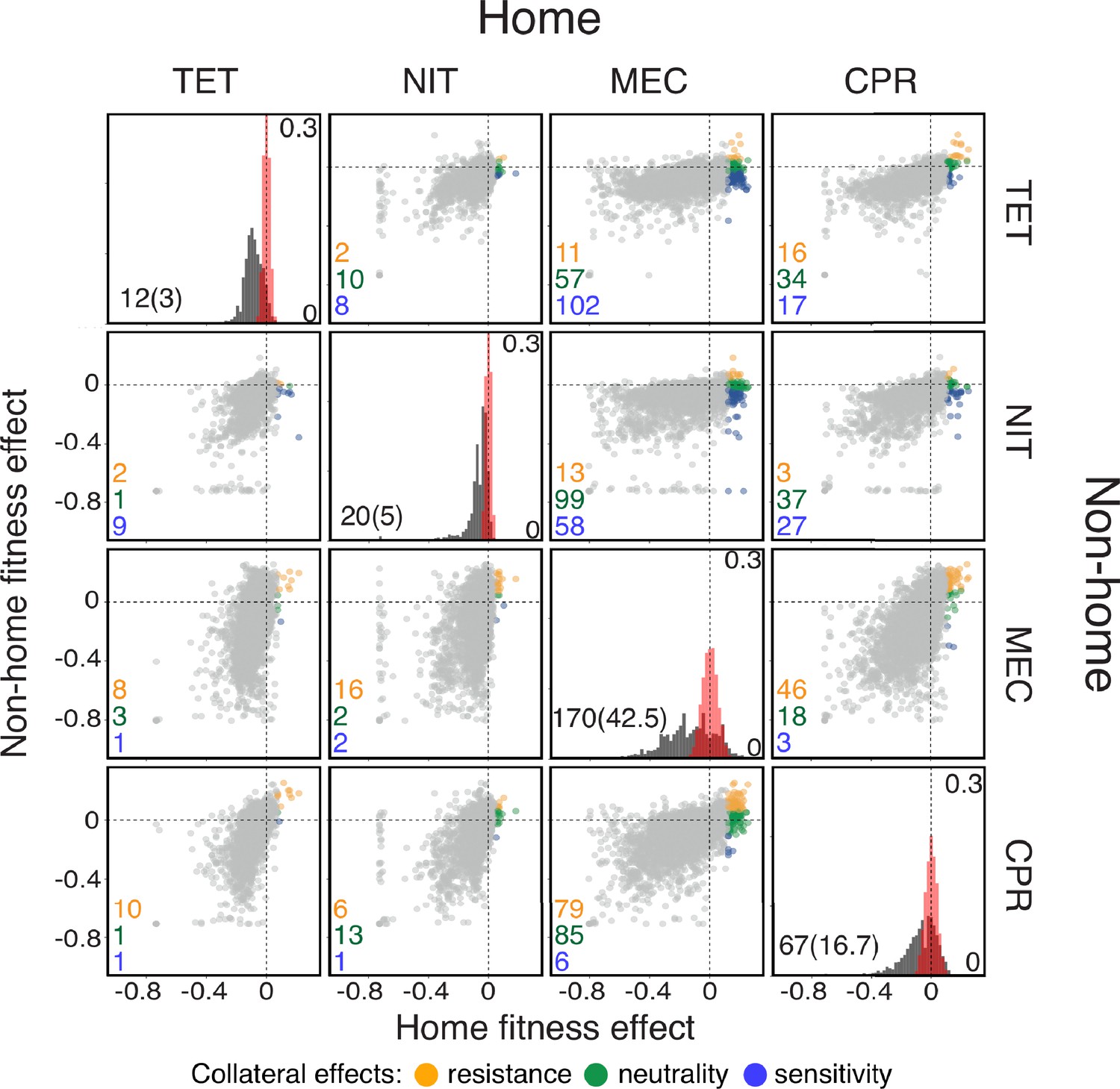
Fitness effects of gene knock-out mutations in E. coli in the presence of four antibiotics.

Data are from Chevereau et al., 2015. Each diagonal panel shows the distribution of fitness effects (DFE) of knock-out mutations in the presence of the corresponding antibiotic (equivalent to Figure 1C in Chevereau et al., 2015). Scale of the $y$ -axis in these panels is indicated inside on the right. The estimated measurement noise distributions are shown in red (see Materials and methods for details). Note that some noise distributions are vertically cut-off for visual convenience. The number of identified beneficial mutations (i.e. resistance mutations) and the expected number of false positives (in parenthesis) are shown in the bottom left corner. The list of identified resistance mutations is given in the Figure 1—source data 1. Off-diagonal panels show the fitness effects of knock-out mutations across pairs of drug environments. The $x$ -axis shows the fitness in the environment where selection would happen first (i.e., the ‘home’ environment). Each point corresponds to an individual knock-out mutation. Resistance mutations identified in the home environment are colored according to their collateral effects, as indicated in the legend. The numbers of mutations of each type are shown in the corresponding colors in the bottom left corner of each panel. TET: tetracycline; NIT: nitrofurantoin; MEC: mecillinam; CPR: ciprofloxacin.

Figure 1—source data 1 P-values and calls of collateral effects of beneficial knock-out mutations in the Chevereau et al., 2015 data (see Materials and methods for details).: https://cdn.elifesciences.org/articles/73250/elife-73250-fig1-data1-v2.csv
Download elife-73250-fig1-data1-v2.csv
Figure 1—source data 2 Calls of collateral effects of mutations beneficial in CTX in the Stiffler et al., 2015 data (see Materials and methods for details).: https://cdn.elifesciences.org/articles/73250/elife-73250-fig1-data2-v2.csv
Download elife-73250-fig1-data2-v2.csv

Figure 1—figure supplement 1

Download asset Open asset

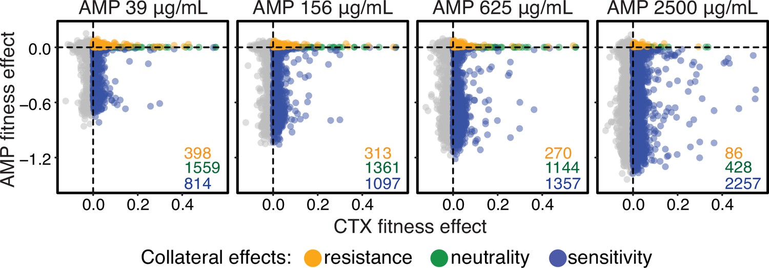
JDFEs of single point mutations in TEM-1 β-lactamase gene in E. coli in the presence of cefotaxime and ampicillin.

Fitness effects of single point mutations in the TEM-1 β-lactamase gene in E. coli in the presence of cefotaxime and ampicillin. Data from Stiffler et al., 2015. Panels show data for different concentrations of ampicillin, as indicated. Fitness is measured as the change in the log ratio of the mutant to wildtype frequency during growth in the presence of the drug. Cefotaxime (CTX) is chosen as the home environment (see Materials and methods for details). Each point represents a single point mutation and is colored by its (collateral) fitness effect in the presence of ampicillin, as indicated in the legend. The numbers of mutations with positive fitness in the presence of cefotaxime with different collateral effects are shown in the lower right corner of each panel.

Figure 2 with 1 supplement

Download asset Open asset

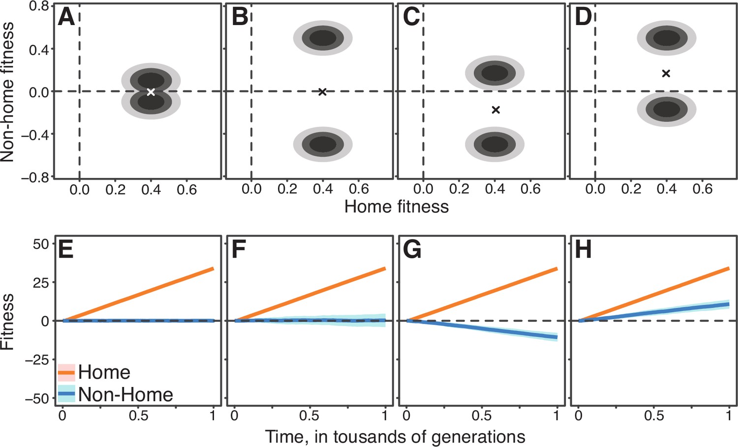
Gaussian JDFEs and the resulting fitness trajectories.

(A–E) Contour lines for five Gaussian JDFEs. ‘‘x’’ marks the mean. For all distributions, the standard deviation is 0.1 in both home- and non-home environments. The correlation coefficient ρ is shown in each panel. (F–J) Home and non-home fitness trajectories for the JDFEs shown in the corresponding panels above. Thick lines show the mean, ribbons show ±1 standard deviation estimated from 100 replicate simulations. Population size $N = 10^{4}$ , mutation rate $U = 10^{- 4}$ ( $U_{b} = 4.6 \times 10^{- 5}$ ).

Figure 2—figure supplement 1

Download asset Open asset

JDFEs with equal probability weights in the first and fourth quadrants and the resulting fitness trajectories.

See Materials and methods for details.

Figure 3 with 1 supplement

Download asset Open asset

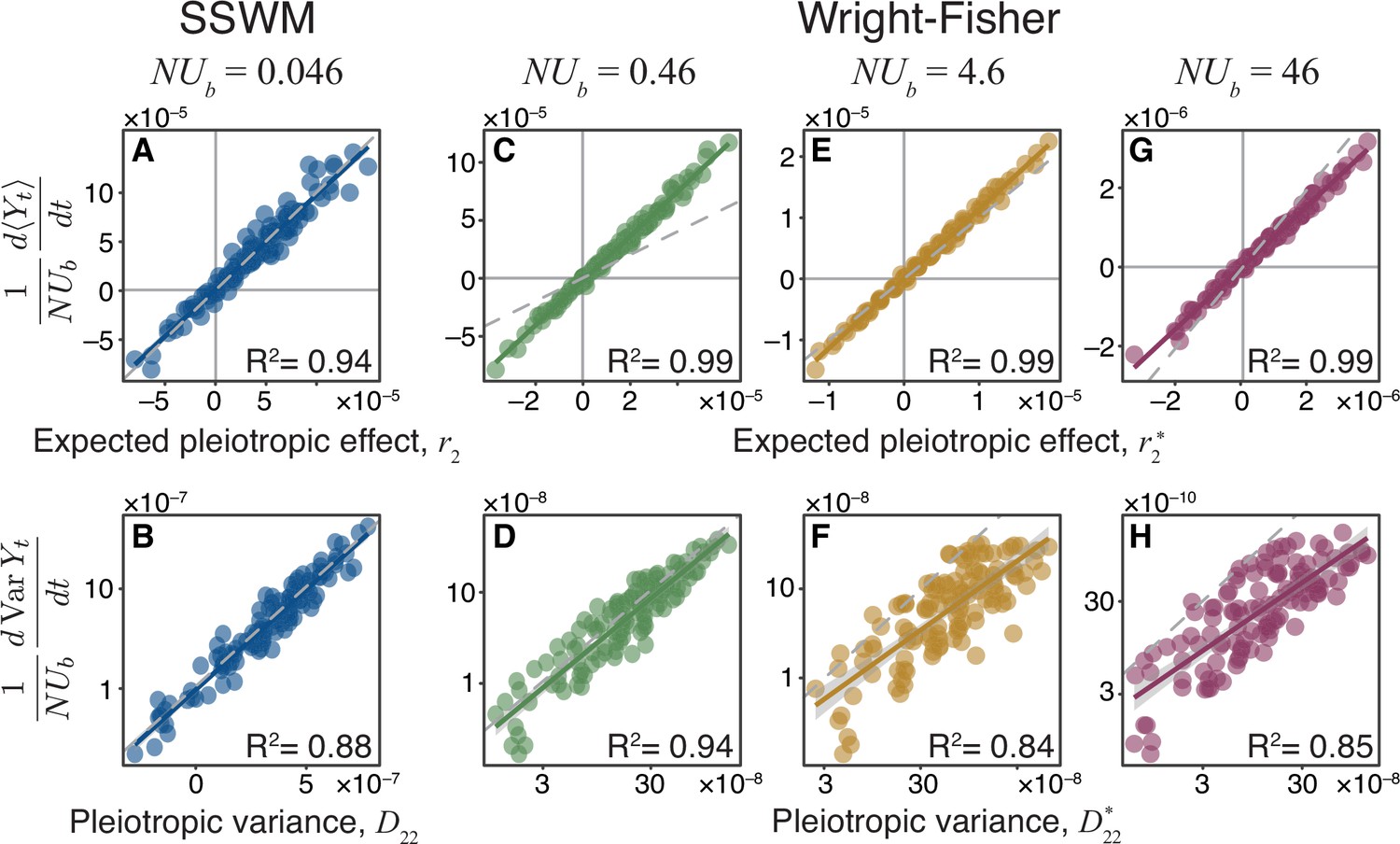
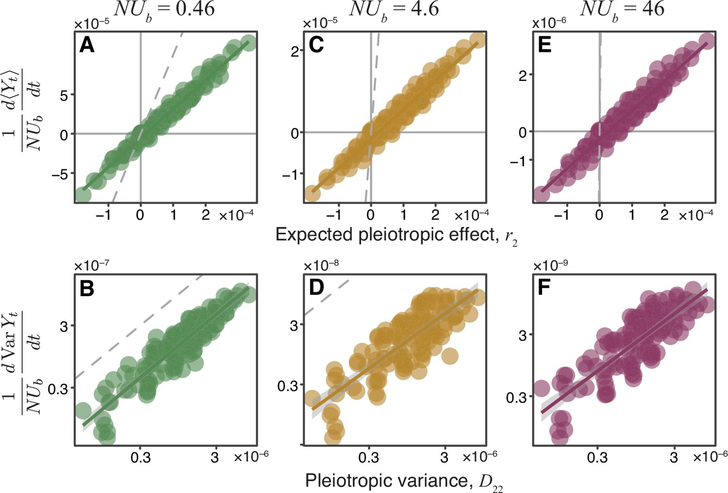
Pleiotropy statistics predict the properties of non-home fitness trajectories in simulations.

Each point corresponds to an ensemble of replicate simulation runs with the same population genetic parameters on one of 125 Gaussian JDFEs (see Figure 3—source data 1 for the JDFE parameters). (A) Expected pleiotropic effect $r_{2}$ versus the scaled slope of the mean rate of non-home fitness change observed in SSWM simulations. (B) Pleiotropic variance $D_{22}$ versus the scaled rate of change in the variance in non-home fitness observed in SSWM simulations. (C, E, G) Expected pleiotropic effect $r_{2}^{*}$ versus the scaled slope of the mean rate of non-home fitness change observed in Wright-Fisher simulations. (D, F, H) Pleiotropic variance $D_{22}^{*}$ versus the scaled rate of change in the variance in non-home fitness observed in Wright-Fisher simulations. (See Figure 3—figure supplement 1 for comparison between simulations and the unadjusted pleiotropy statistics $r_{2}$ and $D_{22}$ ) 1000 replicate simulations were carried out in the SSWM regime. All Wright-Fisher simulations were carried out with $U = 10^{- 4}$ and variable $N$ , 300 replicate simulations per data point (see Materials and methods for details). In all panels, the gray dashed line represents the identity (slope 1) line, and the solid line of the same color as the points is the linear regression for the displayed points ( $R^{2}$ value is shown in each panel; $P §lt; 2 \times 10^{- 16}$ for all regressions).

Figure 3—source data 1 Parameters and summary statistics of simulation results for all Gaussian JDFEs used in Figure 3.: https://cdn.elifesciences.org/articles/73250/elife-73250-fig3-data1-v2.csv
Download elife-73250-fig3-data1-v2.csv

Figure 3—figure supplement 1

Download asset Open asset

Same as Figure 3C-H, but with $r_{2}$ and $D_{22}$ shown on the x-axis.

Figure 4 with 1 supplement

Download asset Open asset

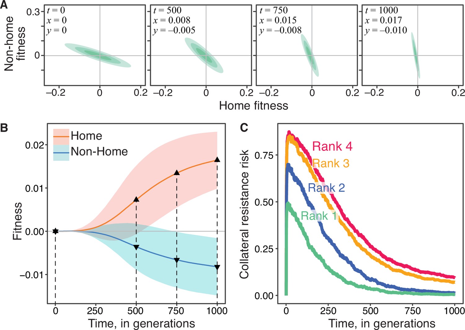
Robust ranking of drug pairs.

(A) Four hypothetical JDFEs, ranked by their $c$ statistic. For all four JDFEs, the mean and the standard deviation in the home environment are $- 1 \times 10^{- 3}$ and $0.01$ , respectively. The mean and the standard deviation in the non-home environment are $1 \times 10^{- 4}$ and $5.1 \times 10^{- 3}$ (rank 1), $2.6 \times 10^{- 3}$ and $7.5 \times 10^{- 3}$ (rank 2), $5.1 \times 10^{- 3}$ and $7.5 \times 10^{- 3}$ (rank 3), $7.5 \times 10^{- 3}$ and $0.01$ (rank 4). Correlation coefficient for all four JDFEs is $- 0.9$ . (B) Collateral resistance risk over time, measured as the fraction of populations with positive mean fitness in the non-home environment. These fractions are estimated from 1000 replicate Wright-Fisher simulation runs with $N = 10^{4}$ , $U = 10^{- 4}$ ( $N U_{b} = 0.46$ ). Colors correspond to the JDFEs in panel A. Numbers indicate the -rank of each JDFE. (C) A priori $c$ -rank ( $x$ -axis) versus the a posteriori rank ( $y$ -axis) based on the risk of collateral resistance observed in simulations, for all 125 Gaussian JDFEs and all $N U_{b}$ values shown in Figure 3. Gray dashed line is the identity line. $R^{2}$ values are $0.94, 0.81$ and $0.82$ for $N U_{b} = 0.46, 4.6$ and $46$ , respectively. $P §lt; 10^{- 15}$ for all regressions.

Figure 4—figure supplement 1

Download asset Open asset

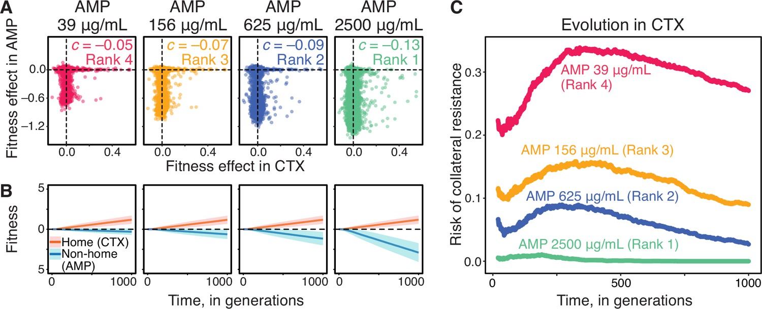
Ranking of AMP concentrations according to their risk of collateral resistance, based on Stiffler et al., 2015 data.

(A) Same as Figure 1—figure supplement 1 but colored by $c$ -rank, as indicated. (B) Home and non-home fitness trajectories for the JDFEs shown in the corresponding panels in A. Notations are as in Figure 2. Population size $N = 10^{4}$ , mutation rate $U = 10^{- 4}$ . (C) Collateral resistance risk over time estimated from 5000 replicate simulations shown in B. Colors correspond to the ranks in A.

Figure 5 with 1 supplement

Download asset Open asset

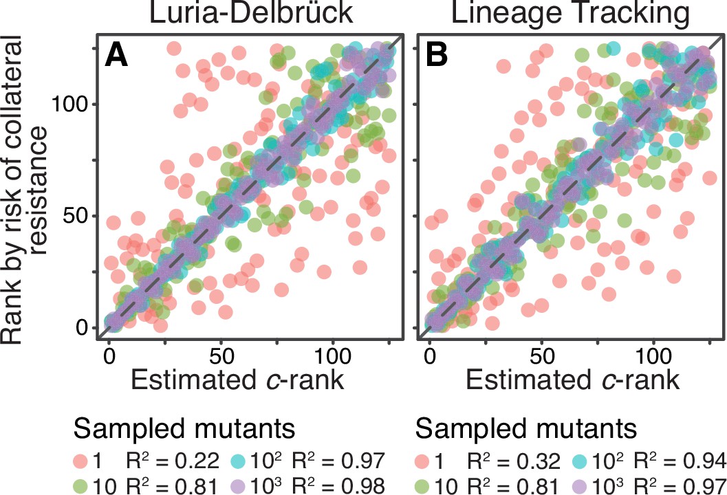
Sampling effects on the ranking of drug pairs.

Both panels show correlations between the a priori estimated $c$ -rank ( $x$ -axis) of the 125 Gaussian JDFEs and their a posteriori rank ( $y$ -axis) based on the risk of collateral resistance observed in simulations (same data as the $y$ -axis in Figure 4C for $N U_{b} = 0.46$ ). (A) The $c$ statistic is estimated using the Luria-Delbrück method (see text for details). Cutoff for sampling mutations is $0.5 σ$ , where σ is the standard deviation of the JDFE in the home environment. See Figure 5—figure supplement 1 for other cutoff values. (B) The $c$ statistic is estimated using the barcode lineage tracking method with $N = 10^{6}$ and $U = 10^{- 4}$ (see text and Materials and methods for details). $P §lt; 10^{- 6}$ for all regressions.

Figure 5—figure supplement 1

Download asset Open asset

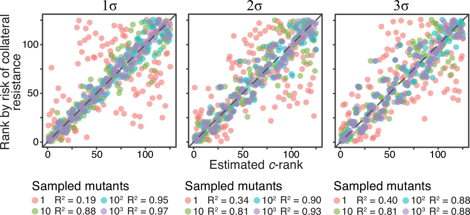
Same as Figure 5A, but with different thresholds for sampling.

Same as Figure 5A, but with different thresholds for sampling mutations, as indicated above each panel (σ is the standard deviation of the JDFE in the home environment). See Materials and methods for details. $P §lt; 10^{- 6}$ for all regressions.

Appendix 1—figure 1

Download asset Open asset

Evolutionon JDFEs with global epistasis and the risk of collateral resistance.

(A) Gaussian JDFE with global epistasis as it changes along the expected evolutionary trajectory shown in panel B. Parameters of the initial JDFE at $x = y = 0$ are the same as for the ank 1 JDFE in Figure 4A; $γ_{h} = γ_{n h} = 0.5$ . (B) Home and non-home fitness trajectories for the JDFE with global epistasis shown in panel A. Thick lines show the mean, ribbons show ±1 standard deviation estimated from 500 replicate simulations. Population size $N = 10^{4}$ , mutation rate $U = 10^{- 4}$ . Dashed vertical lines indicate the time points at which the JDFE snapshots in panel A are shown. (C) Probability of collateral resistance over time for four Gaussian JDFE with global epistasis. Parameters of the initial JDFEs at $x = y = 0$ are the same as for the four JDFE in Figure 4A, and $γ_{h} = γ_{n h} = 0.5$ for all of them. $N = 10^{4}$ , mutation rate $U = 10^{- 4}$ , 1500 replicate simulation runs per JDFE. Colored numbers indicate the predicted -rank of the initial JDFEs (same as in Figure 4A).

Additional files

Transparent reporting form: https://cdn.elifesciences.org/articles/73250/elife-73250-transrepform1-v2.docx
Download elife-73250-transrepform1-v2.docx

Download links

A two-part list of links to download the article, or parts of the article, in various formats.

Downloads (link to download the article as PDF)

Open citations (links to open the citations from this article in various online reference manager services)

Mendeley

Cite this article (links to download the citations from this article in formats compatible with various reference manager tools)

Sarah M Ardell
Sergey Kryazhimskiy

(2021)

The population genetics of collateral resistance and sensitivity

eLife 10:e73250.

https://doi.org/10.7554/eLife.73250

Sign up for email alerts

Privacy notice