Three-dimensional multi-site random access photostimulation (3D-MAP)
- Department of Electrical Engineering & Computer Sciences, University of California, Berkeley, United States
- Department of Molecular & Cell Biology, University of California, Berkeley, United States
- Helen Wills Neuroscience Institute, University of California, Berkeley, United States
- Department of Applied Physical Sciences, University of North Carolina at Chapel Hill, United States
- Department of Biomedical Engineering, University of North Carolina at Chapel Hill, United States
- UNC Neuroscience Center, University of North Carolina at Chapel Hill, United States
Figures
Figure 1 with 2 supplements

Experimental setup for three-dimensional multi-site random access photostimulation (3D-MAP).
(A) A collimated laser beam illuminates the surface of a digital micromirror device (DMD) with a custom illumination angle set by scanning mirrors. The DMD is synchronized with the scanning mirrors to match the 2D mask of the spatial aperture to the illumination angle. (B) Detailed view of the overlapping amplitude masks and illumination angles at the conjugate image plane (green) showing how synchronized illumination angles and amplitude masks can generate a focused spot away from the native focal plane (red). Circular patterns labeled by different colors are spatial apertures projected at different times. The position illuminated by all beams while sweeping through each illumination angle forms a focus at the shifted focal plane at z=Δz. D is the diameter of the sweeping trace. is the illumination angle. (C) A focus generated by computer generated holography (CGH) stimulates the targeted area (blue) in focus but also stimulates non-targeted areas (red) out of focus. 3D-MAP can stimulate only the targeted areas and avoid non-targeted areas by closing the amplitude apertures along propagation directions that project to non-targeted areas (dashed red line). (D) Multiple foci can be generated simultaneously at various depths by superposition of their perspective projection along each illumination angle. (E) Simulated maximum intensity profile along the z-axis for an increasing number of overlapping beams shows how axial resolution increases with the number of superimposed projection directions. (F) Full-width-half-maximums (FWHMs) of the illumination patterns in (E). The data for a single beam is excluded because it has no axial sectioning ability.
Figure 1—figure supplement 1
Comparison of three-dimensional (3D) spatial resolution of 3D-multi-site random access photostimulation (MAP) versus existing photostimulation approaches.
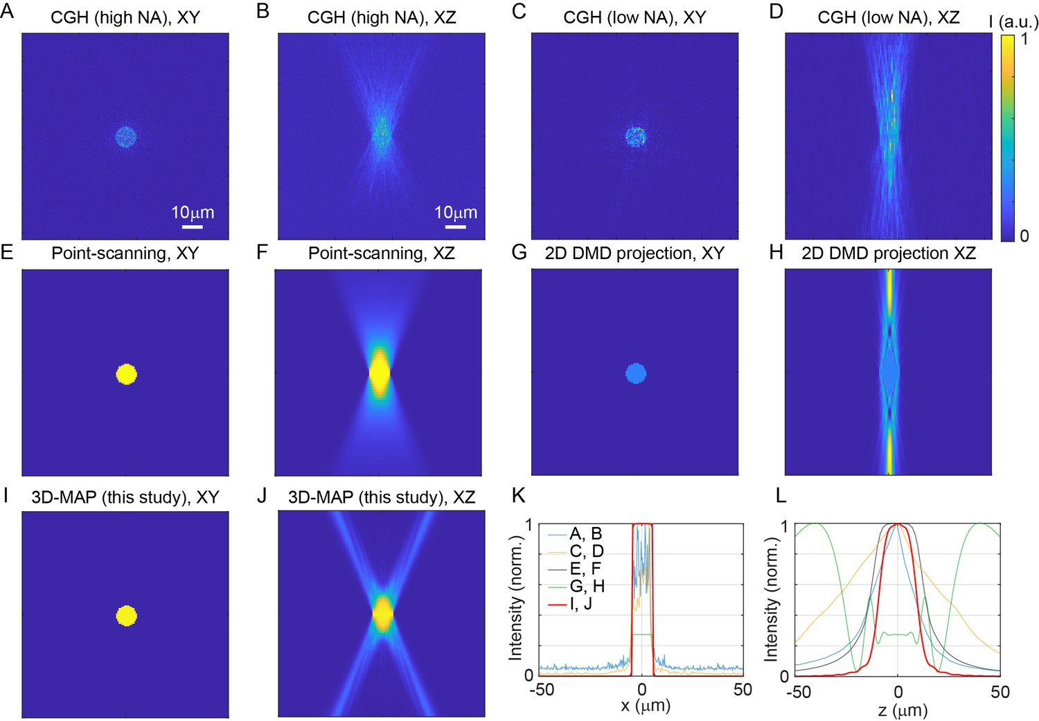
All simulations aim to generate a 10-µm-diameter spot in-focus to match the size of a neuron in order to maximize photostimulation efficiency. The light fields are calculated with 635 nm red light illumination and 20×, NA = 1.0 objective lens. The pixel size of the digital micromirror device (DMD) is 7.5 µm. The number of pixels of the spatial light modulator (SLM) for computer generated holography (CGH) is 1152 × 1152 pixels. (A, B) The lateral cross-section (A) and axial cross-section (B) of CGH at NA = 1.0 (overfill the back aperture). The field-of-view (FOV) under high NA illumination is 319 × 319 µm2, which is much smaller than the FOV of 3D-MAP. (C, D) The lateral cross-section (C) and axial cross-section (D) of CGH at effective NA = 0.55 (under-fill the back aperture) to match the FOV of 3D-MAP (800 × 800 µm2). (E, F) The lateral cross-section (E) and axial cross-section (F) of spiral scan with a single focus. The total intensity is an incoherent sum of the intensity of each scanning point. (G, H) The lateral cross-section (G) and axial cross-section (H) of 2D DMD projection. (I, J) The lateral cross-section (I) and axial cross-section (J) of 3D-MAP (10 overlapping beams). (K, L) A comparison of intensity profile of all these methods along the x-axis (K) and z-axis (L). 3D-MAP achieves the highest 3D spatial resolution among all the methods. Figure (A–J) are in the same size of 100 × 100 µm2. Scale bar, 10 µm.
Figure 1—figure supplement 2
Three-dimensional multi-site random access photostimulation (3D-MAP) can automatically remove illumination angles in non-targeted areas.
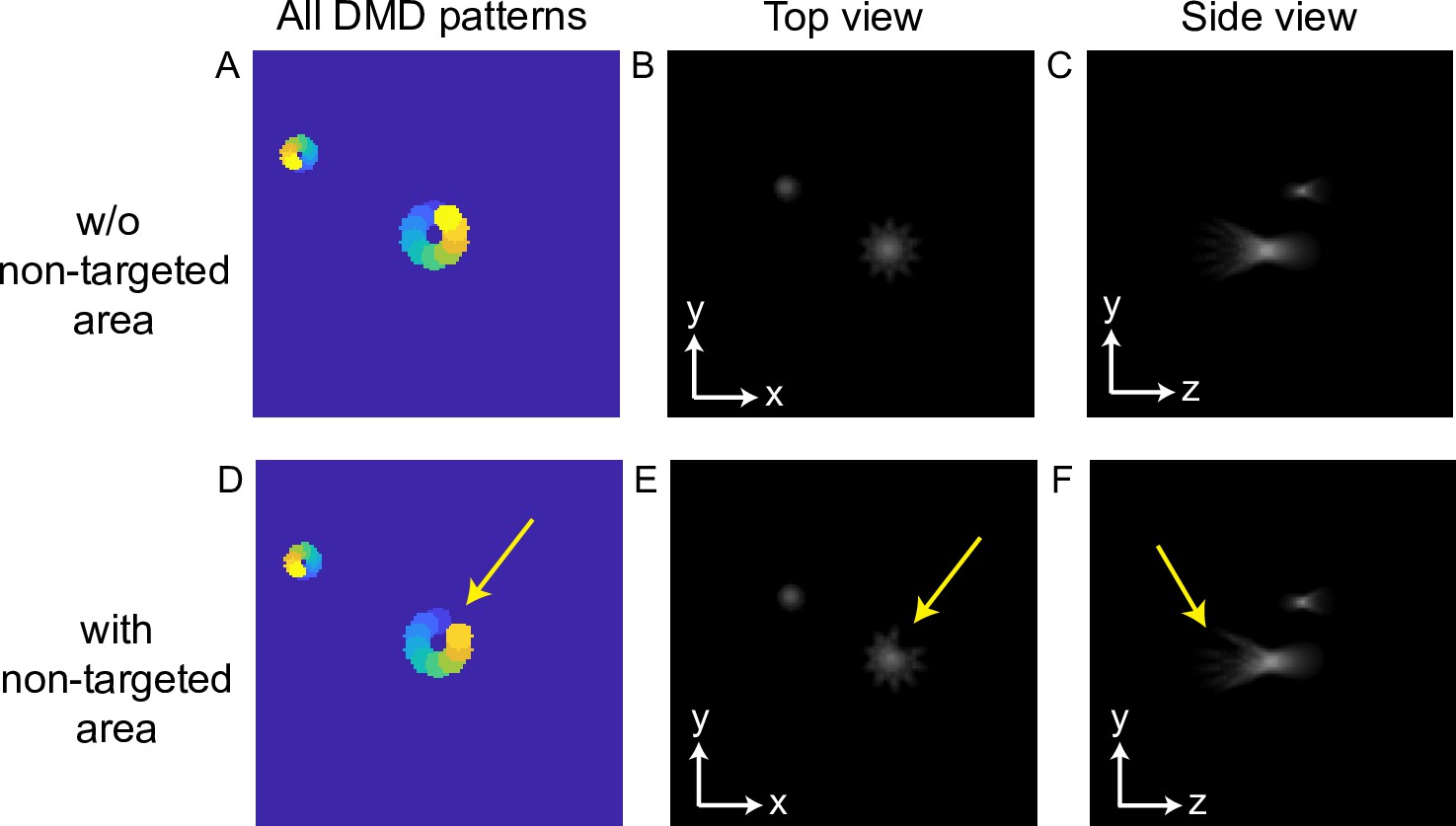
(A–C) The case without non-targeted areas. (D–F) The case with a non-targeted area near the center. (A, D) Overlapping all digital micromirror device (DMD) patterns corresponding to 10 illumination angles. Apertures in the same color are turned on together. Notice that only one yellow aperture is turned on in (D) to generate the small spot, and the other yellow aperture for the big spot (A) is closed due to the non-targeted area. (B, E) Top view of the two spots. (C, F) Side view of the two spots.
Figure 2 with 1 supplement
Optical characterization of the spatial resolution of three-dimensional multi-site random access photostimulation (3D-MAP) under increasing optical scattering conditions.
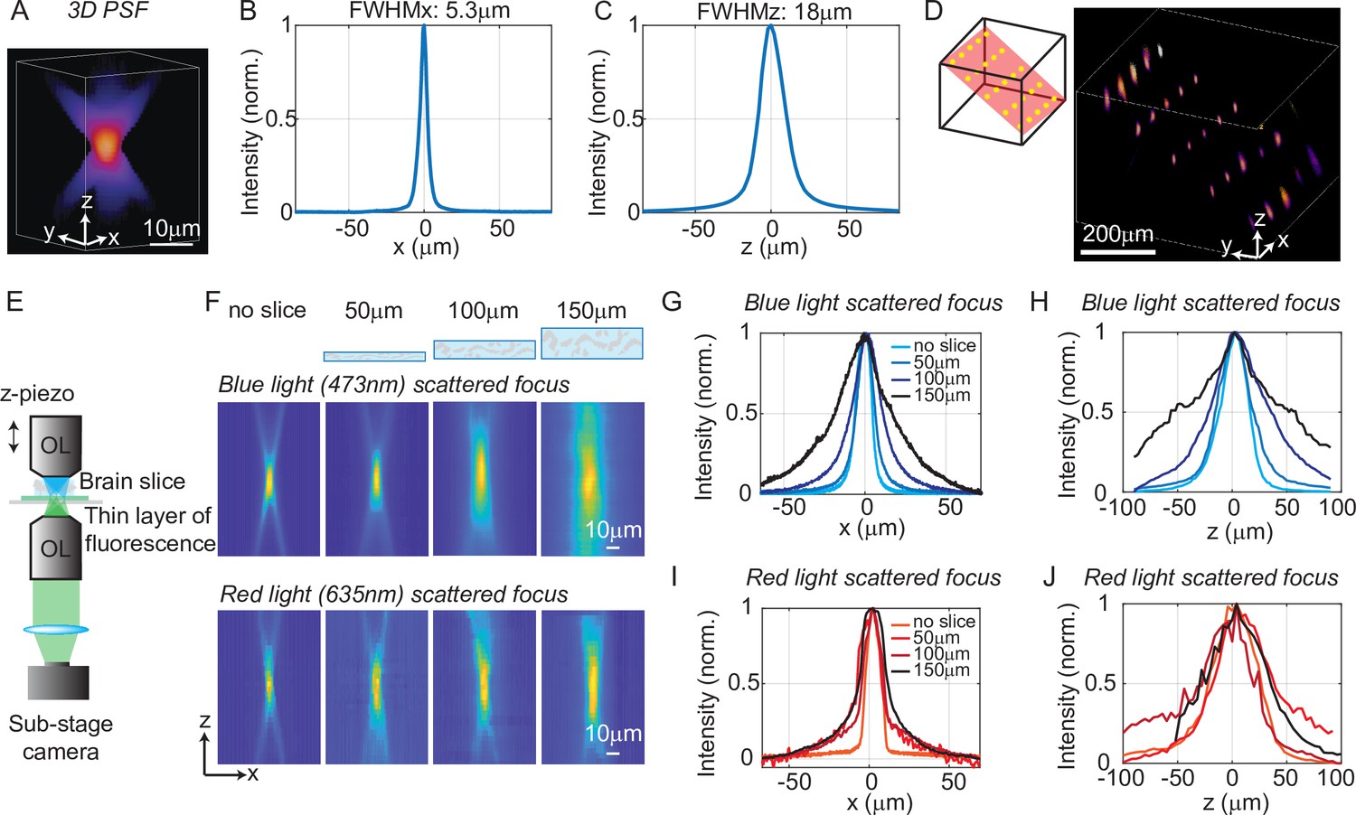
(A) Experimentally measured 3D optical point spread function (PSF) (1-pixel aperture on DMD) built from focus-stacked 2D images of a thin, uniform fluorescent calibration slide recorded at different depths using a sub-stage camera. (B) The PSF’s lateral cross-section (x-axis) has a full-width-half-maximum (FWHM) of 5.3 μm. (C) The PSF axial cross-section (z-axis) has an FWHM of 18 μm. (D) Left: we simultaneously generated 25 foci within a 744 × 744 × 400 μm3 volume. Right, experimental measurement of the corresponding 3D fluorescence distribution. (E) Schematic diagram of the sub-stage microscope assembly for 3D pattern measurement. (F) XZ cross-section of the PSF, measured with blue (473 nm) and red (635 nm) light stimulation without scattering, and through brain tissue slices of increasing thickness: 50, 100, and 150 μm. (G) Under blue light illumination, the FWHM along the x-axis for increasing amounts of scattering is 11.7, 12.2, 19.7, and 29.0 μm, and (H) the FWHM along the z-axis is respectively 42, 46, 76, and 122 μm. (I) With red light illumination, the FWHM along the x-axis for increased amounts of scattering is 10.4, 19.3, 26.7, and 29.6 μm, and (J) the FWHM along the z-axis is respectively 50.7, 75.4, 79.7, and 73.1 μm.
Figure 2—figure supplement 1
Three-dimensional multi-site random access photostimulation (3D-MAP) is able to simultaneously generate multiple foci anywhere in 3D.
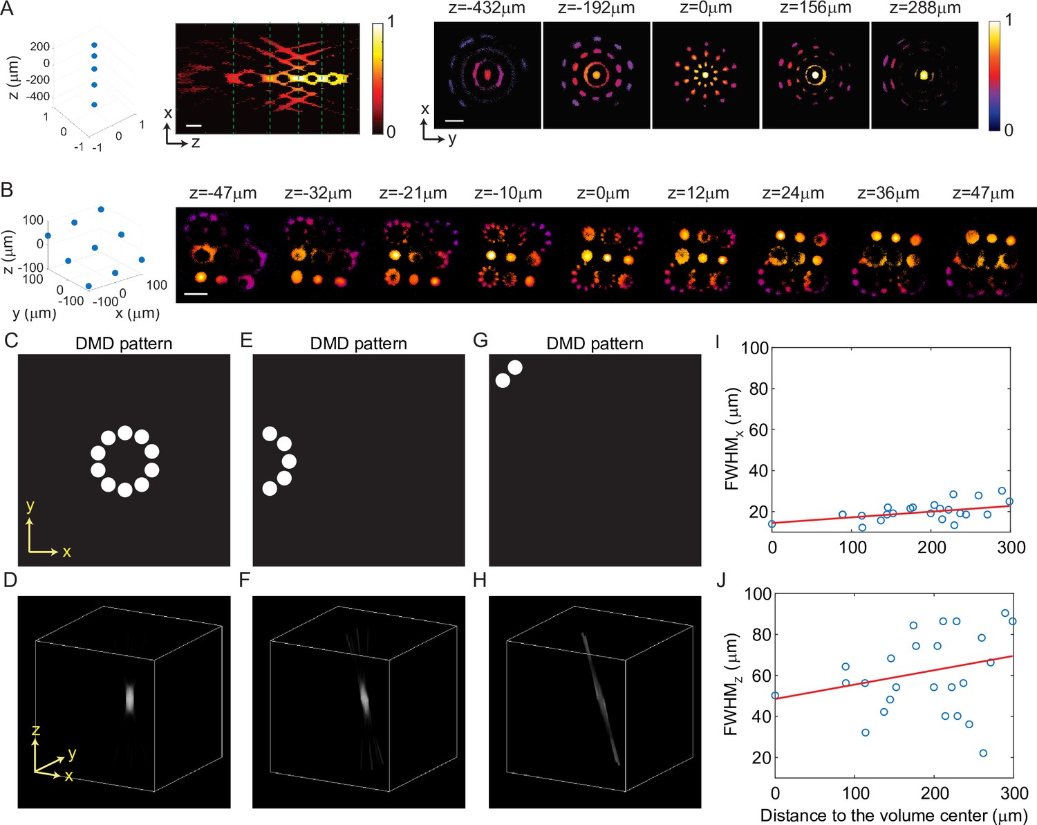
(A) Five foci are located right on top of each other along the z-axis. Left: XZ cross-section. Right: XY cross-section corresponding to the z depths marked with green dash lines. (B) Nine foci with evenly distributed depths form a tilted plane across the 3D volume. For both (A) and (B), the target location is indicated in the 3D diagram on the left, and the corresponding experimental 3D fluorescence measurements are on the right. The foci are recorded in 3D by capturing a stack of 2D fluorescence images at various depths of the 3D illumination pattern intercepting a thin, uniform, fluorescent calibration slide with a sub-stage objective coupled to a camera. Scale bar, 100 μm. (C–H) Simulation results show spatial resolution degrades near the edge of the field-of-view. (C) The digital micromirror device (DMD) pattern to generate a focus in the center of the field-of-view. (D) A focus generated by the 10 beams in C in the center of the accessible volume. (E) The DMD pattern to generate a focus on the edge of the field-of-view. (F) The focus generated by the five beams in E, which is distorted like a coma aberration. (G) The DMD pattern to generate a focus in the corner of the field-of-view. (H) The focus generated by the two beams in G, which is severely distorted and barely has any z-sectioning ability. (I–J) The (I) lateral and (J) axial resolution of the 25 foci showing in Figure 2D versus their distance to the center of the volume. The blue circles mark the full width at half maximum (FWHM) of the foci, and the red line is a linear fitting result. On average, the FWHM of the foci 300 μm away from the center is worse than the one in the center, with (I) 63% worse along the x-axis and (J) 38% worse along the z-axis.
Figure 3 with 1 supplement
Three-dimensional multi-site random access photostimulation (3D-MAP) enables high spatial resolution photo-activation of neurons in vitro and in vivo.
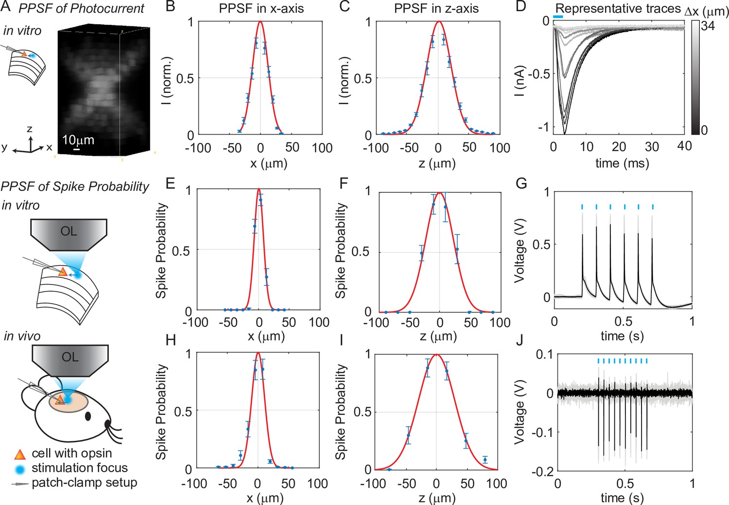
(A) Example 3D representation of a physiological point spread function (PPSF) photocurrent measurement in vitro. (B, C) Photocurrent resolution (full-width-half-maximum [FWHM]) is 29 ± 0.8 μm laterally and 44 ± 1.6 μm axially (n = 9 neurons). (D) Representative traces of direct photocurrent from 11 positions along the x-axis without averaging. (E, F) 3D-MAP evoked spiking resolution in brain slices is 16 ± 2.4 μm laterally and 44 ± 8.9 μm axially (n = 5 neurons). (G) Representative traces of spike probability of 1 for in vitro measurements. (H, I) 3D-MAP evoked spiking resolution measured in vivo is 19 ± 3.7 μm laterally and 45 ± 6.1 μm axially (n = 8 neurons). (J) Representative traces of spike probability of 1 for in vivo measurements. The data shows the mean ± s.e.m. (standard error of the mean) for plots B–C, D–F, and H–I.
Figure 3—figure supplement 1
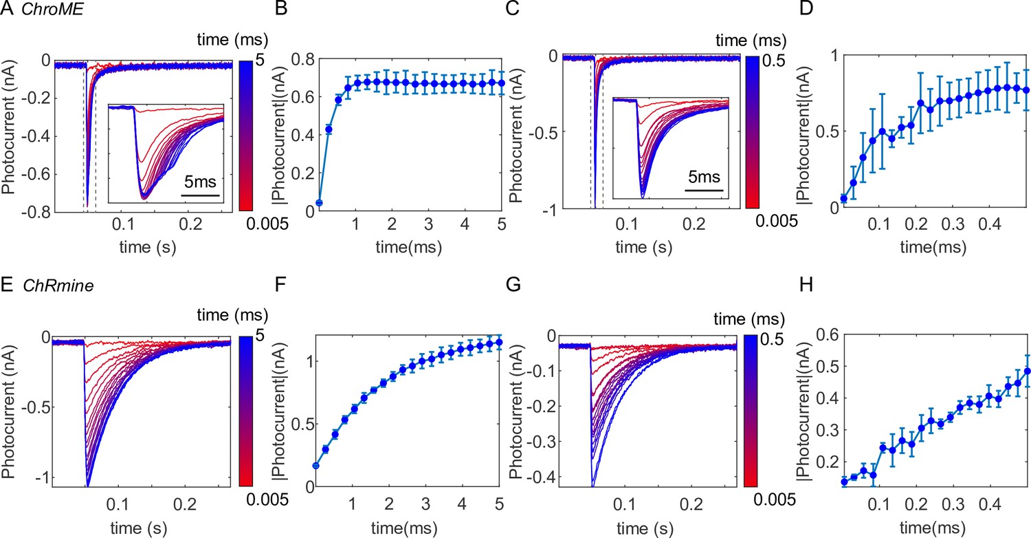
Temporal response of (A–D) ChroME and (E–H) ChRmine, expressed in CHO cells.
(A, E) Photocurrent measured under various stimulation times (i.e., dwell time) ranging from 5 to 5 ms. We used an acousto-optic deflector (AOD) as a fast shutter to control the stimulation time. Insert plot: the zoom-in view of the photocurrent from 0.045 to 0.06 s (dash box). (B, F) The maximum photocurrent at each stimulation time. (C, G) Photocurrent measured at various short stimulation times ranging from 5 to 500 μs. Insert plot: the zoom-in view of the photocurrent from 0.045 to 0.06 s (dash box). (D, H) The maximum photocurrent at each short stimulation time. The result shows the photocurrent of opsins linearly increases with the increase of stimulation time, and gradually saturates at longer stimulation time. The saturation stimulation time is about 0.2 ms for ChroME and about 2 ms for ChRmine. ChroME also has a faster response than ChRmine. Therefore, over kHz patterning speed like what 3D-MAP achieves could reduce the stimulation time so that it becomes possible to photostimulate much more sites in the same experimental time.
Figure 4 with 1 supplement
Three-dimensional (3D) mapping of excitatory synaptic connections with 3D-multi-site random access photostimulation (3D-MAP).
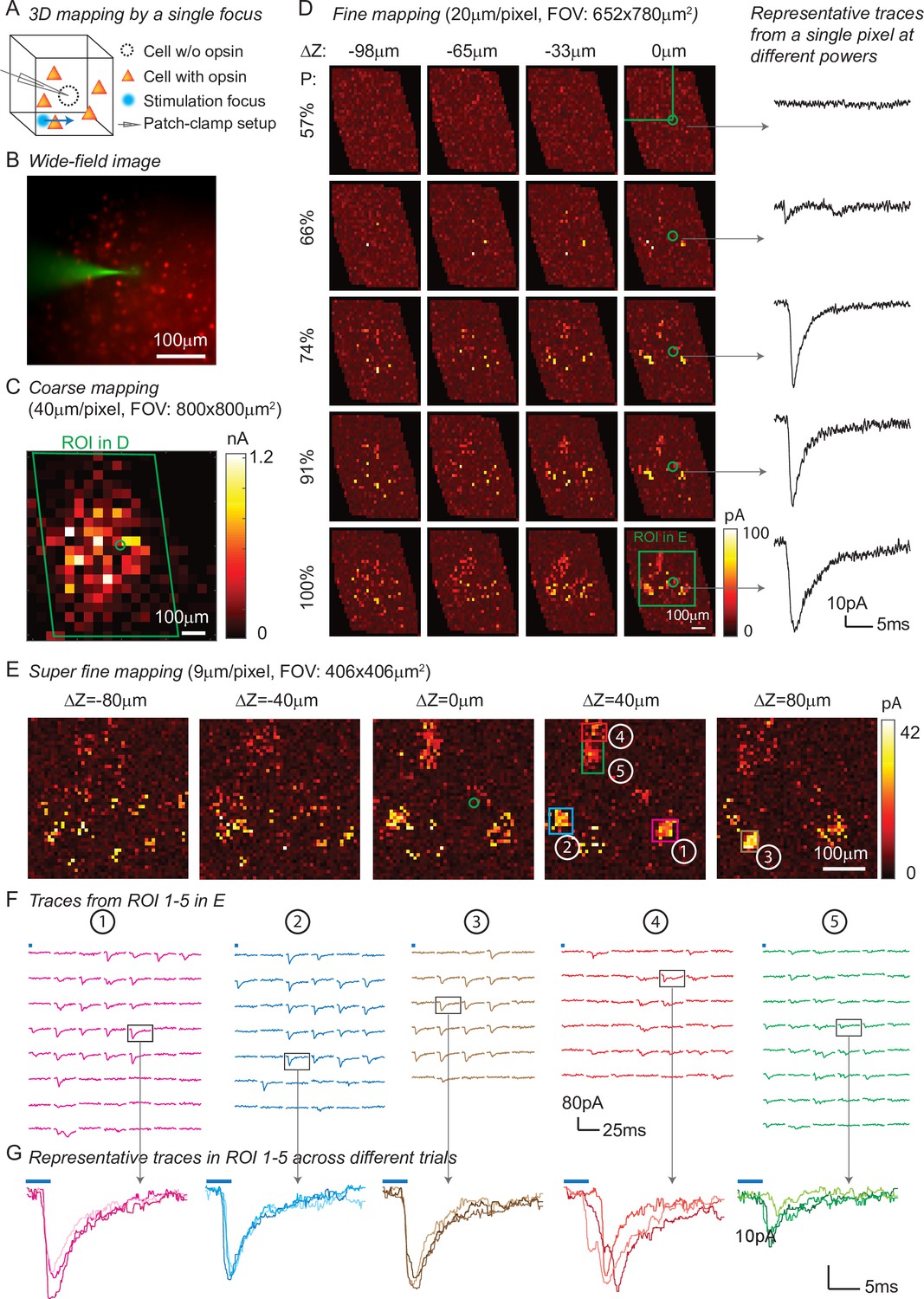
(A) Schematic diagram of the experiment. A single focus randomly scans the volume adjacent to the patched interneuron that does not express opsin, and the readout map reveals the synaptic connections between photo-activated pyramidal neurons and the patched interneuron. (B) An example of widefield image of opsin-expressing pyramidal neurons (red) and the patched interneuron (green). (C) A coarse 2D map in an 800×800 μm 2FOV at 40 μm resolution identifies the sub-regions of the brain slice with presynaptic neurons. (D) Mapping the selected region at higher resolution (green box in C). Each row uses the same stimulation laser power 100% power: 145 μW across multiple axial planes, and each column is a map of the same axial plane at different powers. Representative excitatory postsynaptic currents EPSCs traces right show how synaptic currents at the same photostimulation pixel change as the stimulation power increases, presumably due to recruitment of additional presynaptic neurons. Data are averaged over 5 repetitions. (E) Super-fine resolution mapping of the region of interest (ROI) (green box in D) in 3D at P=90 μW. The green circle in c-e labels the location of the patched interneuron. (F) Traces from ROIs 1-5 labeled in E, averaged over 5 repetitions. (G) Representative traces of single trials without averaging from corresponding ROIs in the same color, measured across three different repetitions. The blue bar on top of traces in F-G indicates the 4ms stimulation time.
Figure 4—figure supplement 1
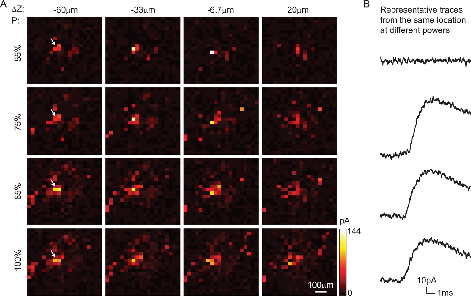
Three-dimensional multi-site random access photostimulation (3D-MAP) provides mapping of inhibitory synaptic connections in vivo.
We patched a pyramidal neuron without opsin at [0, 0, 0] and photostimulated the volume around it pixel-by-pixel, and the parvalbumin neurons connect to this patched cell via synapses expressed opsin. The current readout reveals the inhibitory synaptic connections from all parvalbumin neurons to this pyramidal neuron. The mapping process is repeated four times. (A) Each row of the images is measured under the same stimulation laser power (100% power is 419 μW), and each column of the images is at the same axial plane. Scale bar: 100 µm. (B) Representative traces of postsynaptic currents under each stimulation power (measured from the pixel pointed by white arrow). These traces elucidate the synaptic connection is binary: once the neuron is photostimulated, the synaptic current remains the same, even if the stimulation power is increased. The unique photosensitivity of each neuron helps us to identify different neural ensembles by changing the stimulation power.
Figure 5
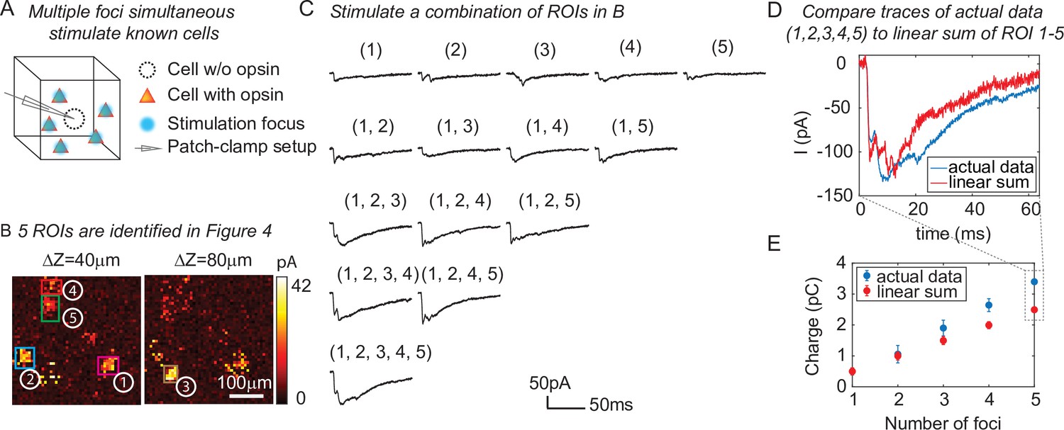
Three-dimensional multi-site random access photostimulation (3D-MAP) is able to stimulate multiple targets simultaneously to explore network dynamics.
(A) Schematic diagram of the experiment. The stimulation ROIs are known to have synaptic connections with the patched interneuron from the widefield mapping as described in Figure 4. (B) The positions of the five ROIs are identified in Figure 4E. (C) Representative photocurrent traces for simultaneous stimulation of subsets of the five ROIs. Traces are averaged over four repetitions. The number(s) above each trace indicate the ROIs that were stimulated to generate the response. (D) Comparison of the actual synaptic response by simultaneous stimulation of ROIs 1–5 (blue) to the response calculated by linearly summing the traces when stimulating ROIs 1–5 individually (red). The individual response from each ROI is shown in the first row of C. (E) Comparison of the integral of the synaptic currents from simultaneous stimulation of multiple connected presynaptic neurons (blue) to the linear sum of the individual stimulation responses (red). The mean and standard deviation of data is calculated from all the k-combinations (number of foci) from the given set of five targets. The sample size is .
Figure 6 with 1 supplement
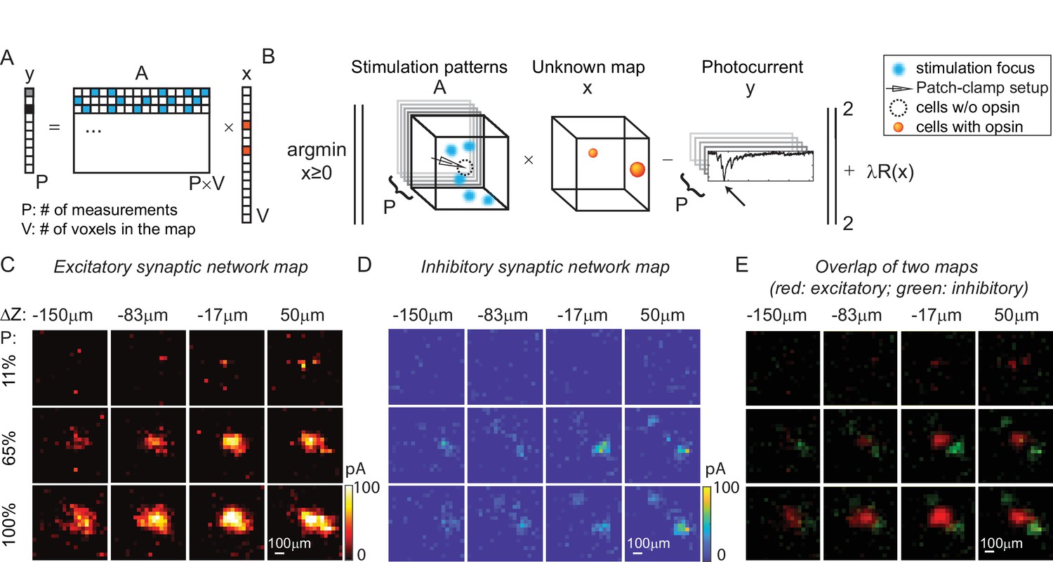
Mapping of synaptic networks in vitro by multi-site random simultaneous stimulation and computational reconstruction.
(A) The forward model for multi-site random simultaneous stimulation. V, the number of voxels in the 3D volume. P, the number of patterns, which are orthogonal to each other. y, peak value of the measured synaptic currents. A is a matrix, where each row represents an illumination pattern, including five foci here (blue, N = 5). x is a vector of the unknown synaptic networks to be reconstructed. (B) Inverse problem formulation. The optimal map, x, minimizes the difference between the peak of measured currents (y) and those expected via the forward model, with a regularizer . (C) Excitatory synaptic connection map of a GABAergic interneuron located at [0, 0, 0]. (D) Inhibitory synaptic connection map from the same cell. (E) Overlap of the excitatory map (red) and inhibitory map (green) to show their spatial relationship. Figures in (C–E) are recorded in an 800 × 800 × 200 µm3 volume at 40 µm/pixel with three different stimulation powers (100% stimulation power is 890 μW in total out of the objective lens). The number of simultaneous stimulation foci (N) is 5 in both cases and the results are average over five repetitions.
Figure 6—figure supplement 1
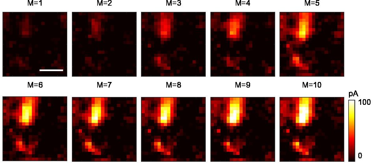
Multi-site random simultaneous stimulation by three-dimensional multi-site random access photostimulation (3D-MAP) can reconstruct synaptic connectivity maps with fewer measurements than single-target stimulation.
M: number of repeat measurements (see Computational reconstruction framework in Materials and methods). The data is recorded from five simultaneously stimulated foci. The optimization problem is underdetermined for values of M < 5. Assuming the five foci stimulate sites which are sparsely distributed in space, it is possible to reconstruct the synaptic connectivity map with fewer measurements (M = 1–4) using compressive sensing. Scale bar, 100 μm.
Figure 7 with 3 supplements
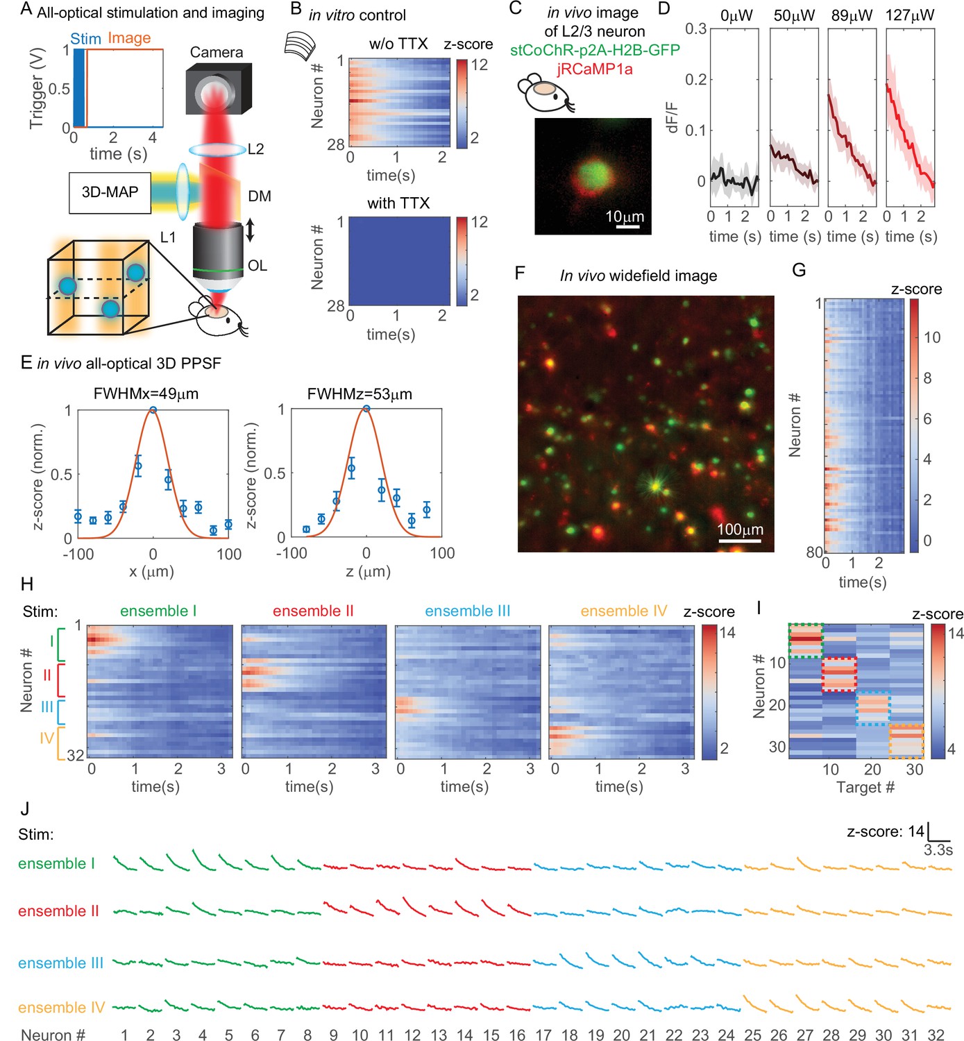
All-optical simultaneous photostimulation and imaging of groups of neurons at L2/3 in the mouse brain.
(A) Experimental setup. The three-dimensional multi-site random access photostimulation (3D-MAP) setup as in Figure 1A is combined with an imaging path using a dichroic mirror, relay lenses, and a camera. Zoom-in view: neurons (blue circles) are stimulated in 3D with 3D-MAP, and calcium activity is recorded from widefield imaging with selective fluorescence excitation (yellow light) by the digital micromirror device (DMD). The dashed plane indicates the imaging focal plane. Top left: a timing plot shows that fluorescence imaging begins at t = 0, immediately after photostimulation. (B) Control experiment with brain slices. Top: calcium activity recorded from 28 neurons. Bottom: same neurons after applying TTX, when no calcium activity is detected. (C) Fluorescent in vivo image of an L2/3 neuron that co-expresses stCoChR-p2A-H2B-GFP (green) and jRCaMP1a (red). (D) Power test of a representative neuron, averaged across 10 repetitions. The blue box indicates the period when stimulation laser is on, and the imaging acquisition is off. (E) In vivo all-optical 3D physiological point spread function (PPSF). The lateral resolution is about 49 ± 21 µm and the axial resolution is about 53 ± 28 µm (n = 10 L2/3 neurons). (F) Maximum z projection of an in vivo widefield image stack (600 × 600 × 40 µm3) of L2/3 neurons (green, stCoChR-p2A-H2B-GFP; red, jRCaMP1a). (G) Calcium activity of 80 neurons as in F recorded during simultaneous photostimulation and imaging. (H) Calcium activity of 32 neurons that are addressed with four distinct photostimulation patterns (labeled with different colors, also see Figure 7—figure supplement 1H) while fluorescence imaging data is acquired. (I) Peak z-score of each calcium trace recorded in H versus the corresponding stimulation patterns. The dashed colored rectangles highlight the neurons that are stimulated in each of the four patterns. (J) Calcium transients of 32 neurons that are stimulated with four distinct patterns, which is the line graph of the same data in (H).
Figure 7—figure supplement 1
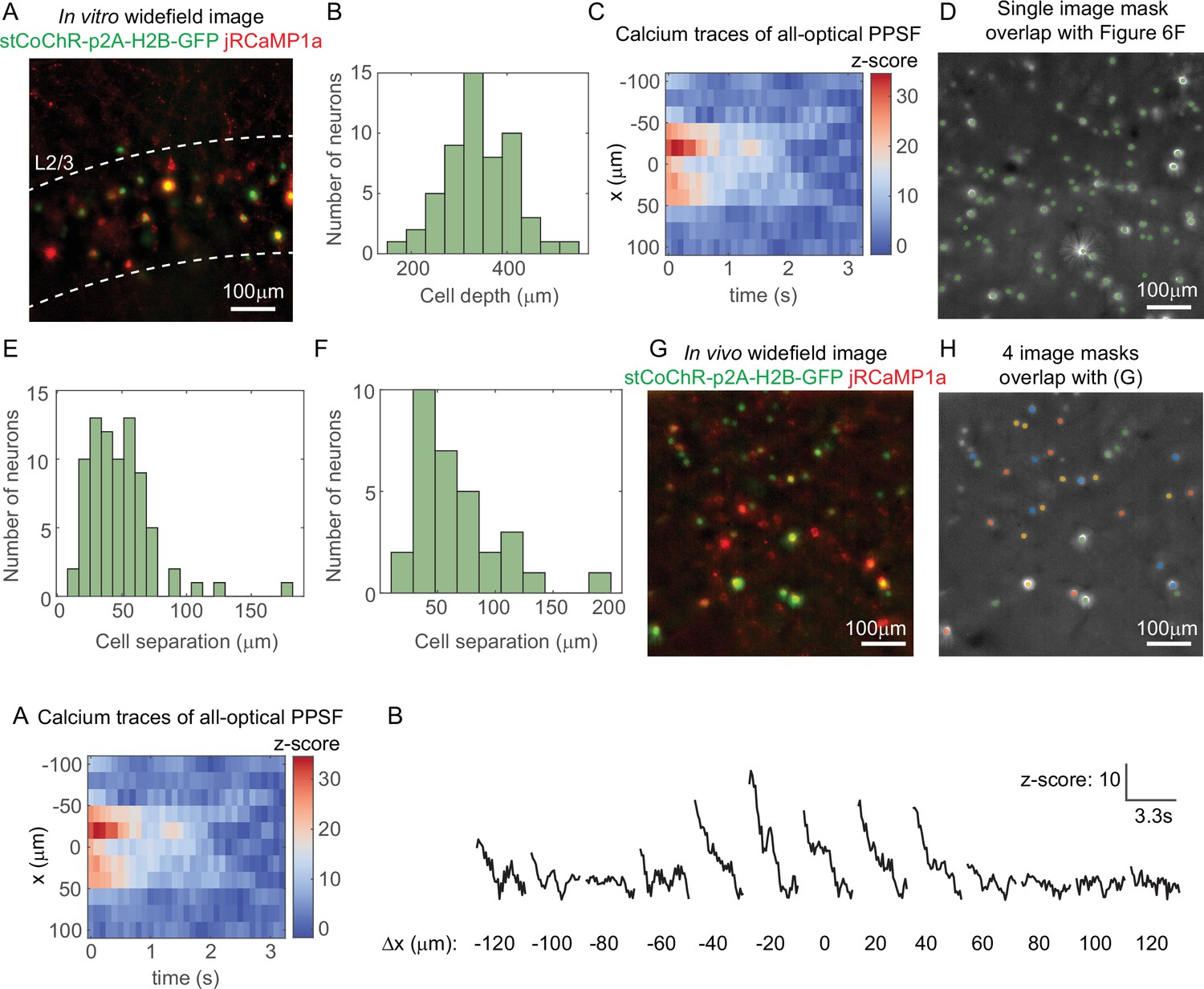
All-optical interrogation of neurons with three-dimensional multi-site random access photostimulation (3D-MAP).
(A) Maximum z projection of the brain slice used in the control experiment (Figure 7B–C). (B) Histogram of the depth of 55 neurons relative to the surface of the mouse brain. The expression is in L2/3. (C) An example of calcium traces at 11 lateral locations (y-axis) in the experiment of in vivo all-optical physiological point spread function (PPSF) measurement. The traces are averaged across 10 repetitions of a represented neuron at x = 0. (D) The image mask on the digital micromirror device (DMD) for the 80 neurons in the volume shown in Figure 7F. Green, the image mask generated by image segmentation. Gray scale image, maximum z projection of the widefield image stack of the somata. (E) Histogram of neuron separation in D. The mean separation of the 80 neurons is 49 ± 26 µm. (F) Histogram of neuron separation in G–H. The mean separation of the 32 neurons is 67 ± 37 µm. (G) Maximum z projection of the in vivo widefield image stack of the neurons in Figure 7H–J. (H) The four different image masks for ensemble stimulation in Figure 7H–J. (I) Line graph of calcium transients in (C). Neurons labeled by the same color are photostimulated simultaneously. The masks are generated by Poisson disc sampling.
Figure 7—figure supplement 2
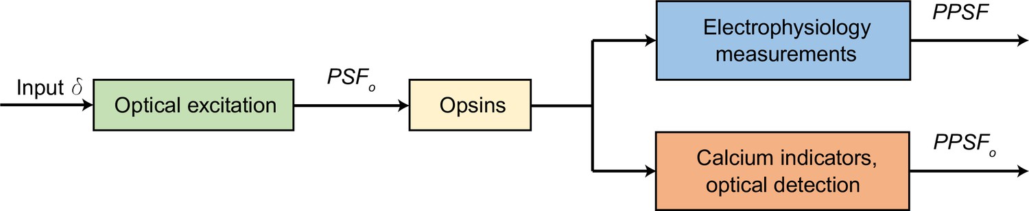
The relation between optical point spread function (PSFo), physiological PSF (PPSF), and all-optical PPSF (PPSFo).
The three PSFs evaluate the response to a point source under different systems. PSFo shows the spatial resolution of the optical system (Figure 2); PPSF measured by electrophysiology (Figure 3) is not only related to the optical system but also to opsin (opsin conductance, the total opsin expression levels, and the intrinsic excitability of the neuron); PPSFo (Figure 7) evaluates the system consisting of optical excitation path, opsin, calcium indicators, and optical detection path. PPSFo in Figure 7E may be similar to the electrophysiology PPSF in Figure 3H–J, despite being 50–100 µm deeper, because jRCaMP1a probably cannot detect very low spike rates. Therefore, each of these various PSFs depends on the specific experiment, which are not expected to be equal.
Figure 7—figure supplement 3
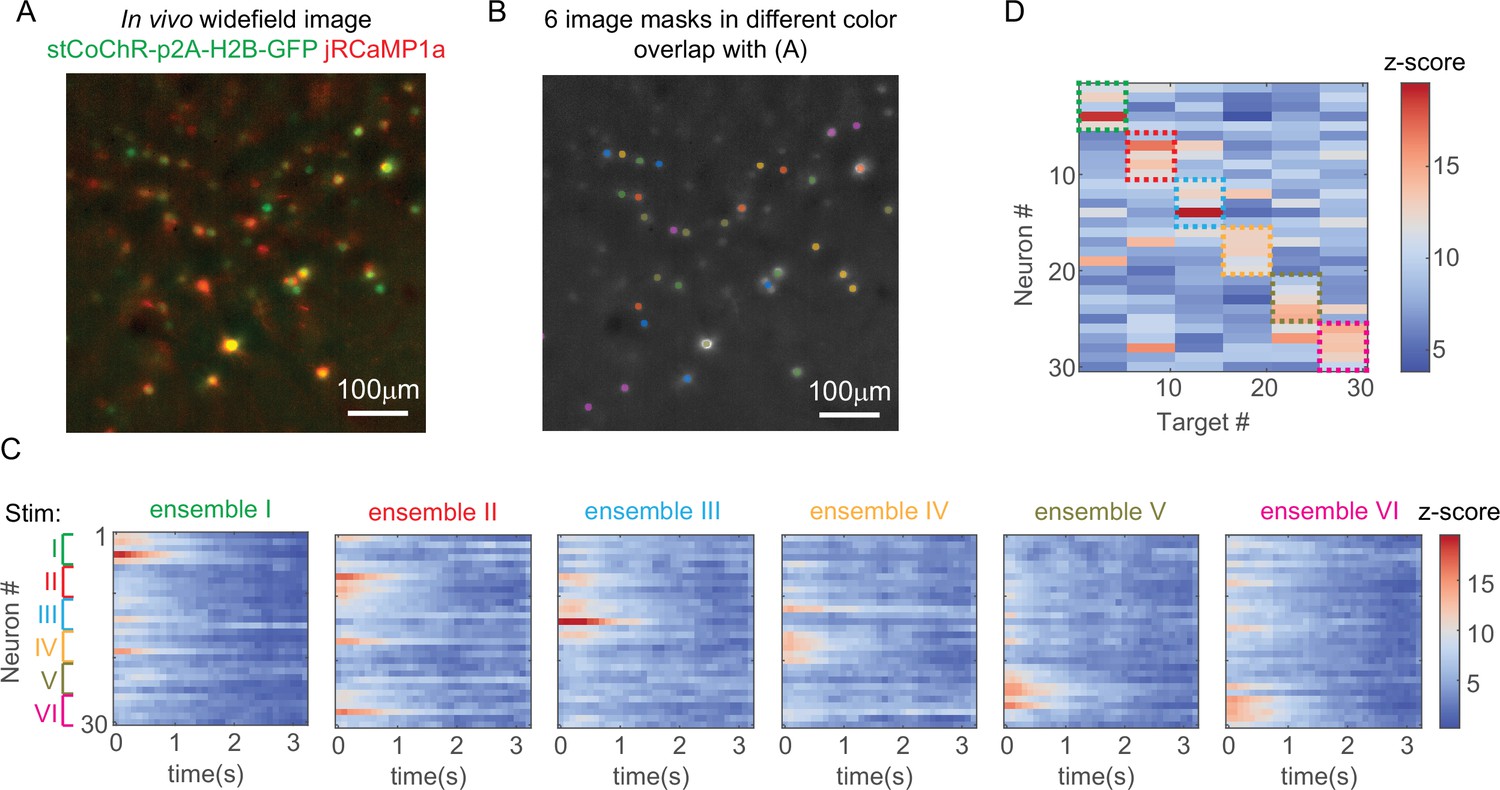
Another example of stimulating ensembles while imaging all the neurons in vivo.
(A) Maximum z projection of the in vivo widefield image stack of the neurons. (B) Six distinct patterns for ensemble stimulation and imaging. (C) Calcium activity of 30 neurons that are addressed with the six patterns in B. (D) Peak z-score of each calcium trace recorded in C versus the corresponding stimulation patterns. The dashed colored rectangles highlight the neurons that are stimulated in each of the six patterns.
Figure 8
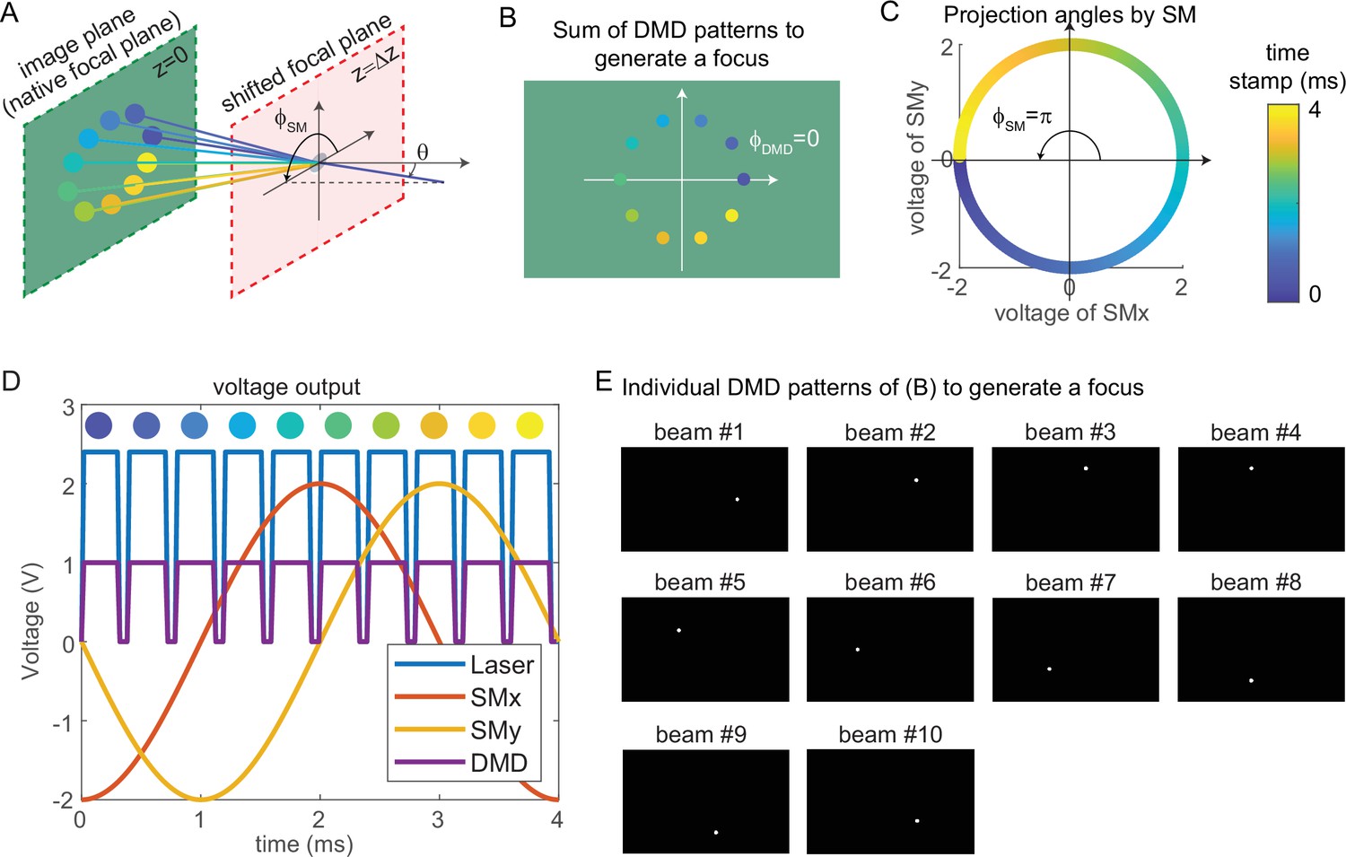
Synchronized control of the scanning mirrors and the digital micromirror device (DMD) to generate a focus at a shifted focal plane by three-dimensional multi-site random access photostimulation (3D-MAP).
(A) A focus spot is generated by 10 beams in 4 ms in total. The DMD is located at the relayed image plane projecting 10 apertures sequentially. Scanning mirrors control the corresponding projection angles for each beam. is the same for all beams and varies. The color of the apertures and the projection angles shows their respective time stamp. (B) 2D view of the image plane in A, showing all 10 apertures on the DMD that are used to generate the focus. The first aperture (dark blue circle) is at and the 10 apertures are evenly distributed in the range of . (C) Projection angles by scanning mirrors. The first projection angle to generate the focus in A with the first aperture in B is located at . The scanning mirrors evenly scan along a circular trace in the 4 ms stimulation time. (D) The voltage outputs control the hardware. The scanning trace in C is generated by applying sinusoidal signals (red, yellow) to the scanning mirrors. The maximum voltage of the sinusoidal signal decides and the phase of the sinusoidal signal decides . The DMD projection is controlled by the TTL signal (purple), which has 10 rising edges in the 4 ms stimulation time to project 10 patterns sequentially. The laser intensity is controlled by an analog signal (blue) that is synchronized with the DMD. (E) The 10 patterns to be projected by the DMD to synthesize the focused spot.
Figure 9
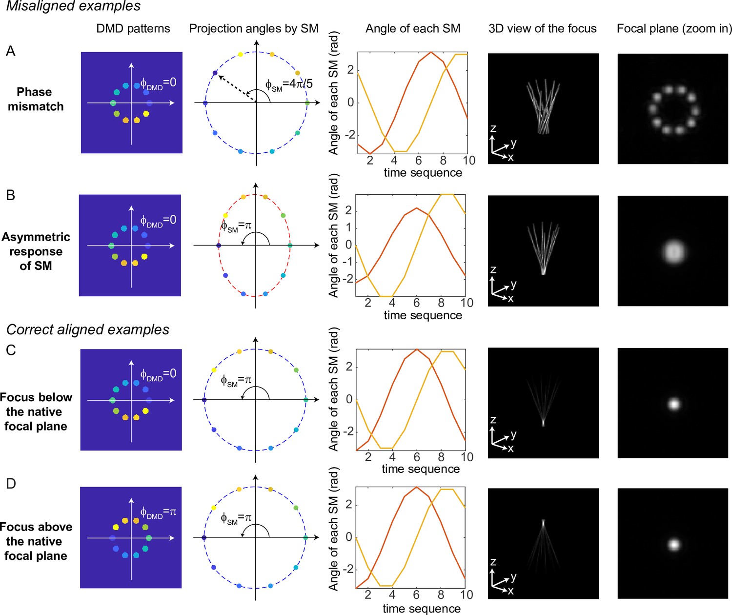
Misaligned examples (A, B) and correct aligned examples (C, D) with three-dimensional multi-site random access photostimulation (3D-MAP).
The first column shows the sum of 10 digital micromirror device (DMD) patterns to generate the focus. The second column shows the projection angles by the scanning mirrors (SM). The color labels the timestamp of the projection as in Figure 7. The third column shows the angle of the scanning mirror in the x-axis (red) and the angle of the scanning mirror in the y-axis (yellow) for the sequential 10 projections, respectively. The fourth column shows the 3D view of the focus (distorted or tightly focused). The fifth column shows the 2D XY-view at the in-focus plane. To show the focus better, the images are zoomed in compared to the images in the fourth column. (A) Misaligned example of phase mismatching. The 10 beams cannot overlap to generate a tight focus, instead, a ring is generated at the shifted focal plane. (B) Misaligned example of asymmetric response of the scanning mirrors. The beams in the tangential direction and in the sagittal direction overlap at different locations along the z-axis like astigmatism, generating a distorted focus. (C) Correct aligned example generates a focus below the native focal plane (same as Figure 7). (D) Correct aligned example generates a focus above the native focal plane by adding a -phase shift to the DMD patterns.
Tables
Appendix 1—table 1
Comparison of light-targeting photostimulation methods.
| Specific technique | Two-photon optogenetics | One-photon optogenetics | |||
|---|---|---|---|---|---|
| Scanning methods (GM and AOD)* | DMD‡ projection | CGH § | Our technique 3D-MAP | ||
| Pros | · High 3D resolution · High penetration depth · Less cross-talk because of non-linear excitation | • Low power illumination • Compact and inexpensive systems | |||
| • Reduced cross-talk with sparse excitation | • Fast patterning speed • Large field-of-view | • High 3D resolution | • Large number of DoF • Fast patterning speed • High 3D resolution • Large field-of-view • Less cross-talk from out-of-focus light | ||
| Cons | • Moderate numbers of targets • Small accessible volume • Small numbers of degrees-of-freedom • High-power illumination (heat and photodamage) • Expensive and sophisticated systems • Slow patterning speed | • Rayleigh scattering limits penetration depth • Lower axial resolution than two-photon optogenetics | |||
| • No simultaneous multiple stimulation • Small number of DoFƗ | • Low resolution • No depth specificity • 2D modulation • Small number of DoF† • Cross-talk from out-of-focus light | • Small number of targets • Small accessible volume • Small number of DoF • Slow patterning speed • Cross-talk from out-of-focus light | • Lossy amplitude modulation that requires bright laser sources | ||
| Refs | Carrillo-Reid et al., 2019; Naka et al., 2019; Daie et al., 2021; Sridharan, 2021; Nikolenko et al., 2008; Papagiakoumou et al., 2010; Pégard et al., 2017 | Robinson et al., 2020; Forli et al., 2021; Mardinly et al., 2018 | Mardinly et al., 2018; Leifer et al., 2011; Adam et al., 2019; Werley et al., 2017; Sakai et al., 2013 | Lutz et al., 2008; Anselmi et al., 2011; Szabo et al., 2014; Reutsky-Gefen et al., 2013 | This study |
-
*
GM: galvo mirrors. AOD: acousto-optic deflectors.
-
†
DoF: degrees of freedom.
-
‡
DMD: digital micromirror device
-
§
CGH: computer generated holography.
Appendix 1—table 2
Comparison of the cost of one-photon 3D-MAP and two-photon 3D-SHOT (Pégard et al., 2017; Mardinly et al., 2018).
| 1P 3D-MAP | 2P 3D-SHOT | |||||
|---|---|---|---|---|---|---|
| Description | Part # | Budget | High performance | Part # | Budget | High performance |
| Photostimulation and imaging lasers | Blue DPSS laser | $700 | $9000 | Femtosecond laser for photostimulation | $80,000 | $160,000 |
| Yellow DPSS laser | $3500 | $13,000 | Femtosecond laser for calcium imaging | $80,000 | $140,000 | |
| Imaging sensor/system | sCMOS camera | $5000 | $25,000 | PMTs and acquisition system | $20,000 | $40,000 |
| Light modulator | DMD and the controller | $2000 | $15,000 | LCoS-SLM | $15,000 | $60,000 |
| Scanning mirrors | $2500 | $6400 | ||||
| Optical table | min 3’×3’ | $4000 | $7500 | min 4’×6’ | $8500 | $10,000 |
| Total | $17,700 | $75,900 | $203,500 | $410,000 | ||
Appendix 1—table 3
Summary of experiment details.
| Figure | Type | Sample | Label | DMD aperture size | Imaging parameters |
|---|---|---|---|---|---|
| Figure 2 | Widefield imaging with a sub-stage camera | Uniform fluorescent calibration slide | Fluorescence paint from Tamiya Color, mouse brain slices are label-free | Figure 2A–C: 1 pixel Figure 2D–J: 10 pixels | Capture one widefield image at each z-plane. Imaging speed: 10 Hz |
| Figure 3 | Photostimulation and electrophysiology | Figure 3A–G: brain slices Figure 3H–J: in vivo | L2/3 excitatory neurons expressing soma-targeted ChroME | Figure 3A–D: 15 pixels Figure 3E–J: 10 pixels | N/A |
| Figure 4 | Figure 4B: widefield fluorescence imaging Figure 4C–G: Photostimulation and electrophysiology | Brain slices | L2/3 excitatory neurons expressing soma-targeted ChroME | Figure 4C: 50 pixels Figure 4D–G: 20 pixels | Captured one widefield image. Exposure time: 100 ms |
| Figure 5 | Photostimulation and electrophysiology | Brain slices | L2/3 excitatory neurons expressing soma-targeted ChroME | Figure 5C–D: 20 pixels | N/A |
| Figure 6 | Photostimulation and electrophysiology | Brain slices | L2/3 excitatory neurons expressing Chrimson | Figure 6C–E: 10 pixels | N/A |
| Figure 7 | Photostimulation and calcium imaging | Figure 7B: brain slices Figure 7C–I: in vivo | L2/3 excitatory neurons co-expressing soma-target CoChR and red calcium indicator jRCaMP1a | Figure 7B–I: 10 pixels | Exposure time: 3.8 s Imaging speed: 10 Hz |
Additional files
Download links
A two-part list of links to download the article, or parts of the article, in various formats.
Downloads (link to download the article as PDF)
Open citations (links to open the citations from this article in various online reference manager services)
Cite this article (links to download the citations from this article in formats compatible with various reference manager tools)
Three-dimensional multi-site random access photostimulation (3D-MAP)
eLife 11:e73266.
https://doi.org/10.7554/eLife.73266


