Different computations over the same inputs produce selective behavior in algorithmic brain networks
- School of Psychology and Neuroscience, University of Glasgow, United Kingdom
- Department of Psychology, Edge Hill University, United Kingdom
Figures
Figure 1 with 4 supplements
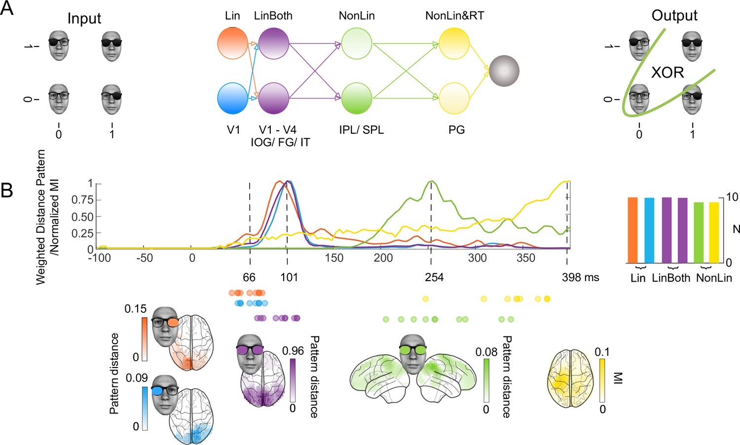
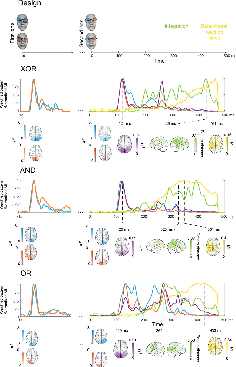
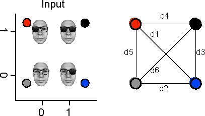
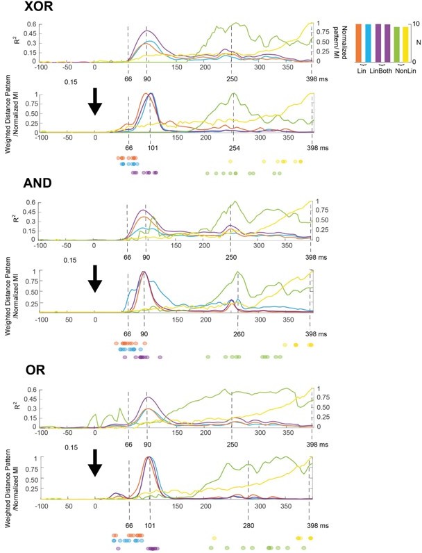
XOR task, four stages of computation in a schematic network and in the brain.
(A) Hypotheses and schematic hierarchical brain network in the XOR task. Stimuli consisted of the image of a face wearing glasses, with dark (‘1’, ‘on’) and clear (‘0’, ‘off’) left and right lenses serving as inputs, for a total of four input classes for XOR behavioral decisions. (B) Four hierarchical stages of computations. Each colored curve shows the average (N = 10 participants) time course of the maximum across sources that: (1) linearly discriminates in its magnetoencephalographic (MEG) activity the ‘on’ vs. ‘off’ state of the left (Lin, blue) and right (Lin, orange) inputs (weighted distance pattern), (2) linearly discriminates both inputs (LinBoth, magenta) (weighted distance pattern), (3) nonlinearly integrates both inputs with the XOR task pattern (NonLin, green) (weighted XOR pattern metric) and (4) nonlinearly integrates both inputs with the XOR task pattern and with amplitude variations that relate to reaction time (RT) (mutual information, MI (MEG; RT)) (yellow). Colored brains localize the regions where these computations start (onset times for left and right) or peak (peak latencies for both, XOR and RT) (p<0.05) familywise error rate corrected with a permutation test, (see Methods, Linear vs. Nonlinear Representations; Representation Patterns). Dots report the onset time of computation (1) and (2) and the peak time of computation (3) and (4) in each participant. See Table 2 and Figure 1—figure supplement 2 for individual participant replications of each computation in the same brain regions and time windows.
Figure 1—figure supplement 1
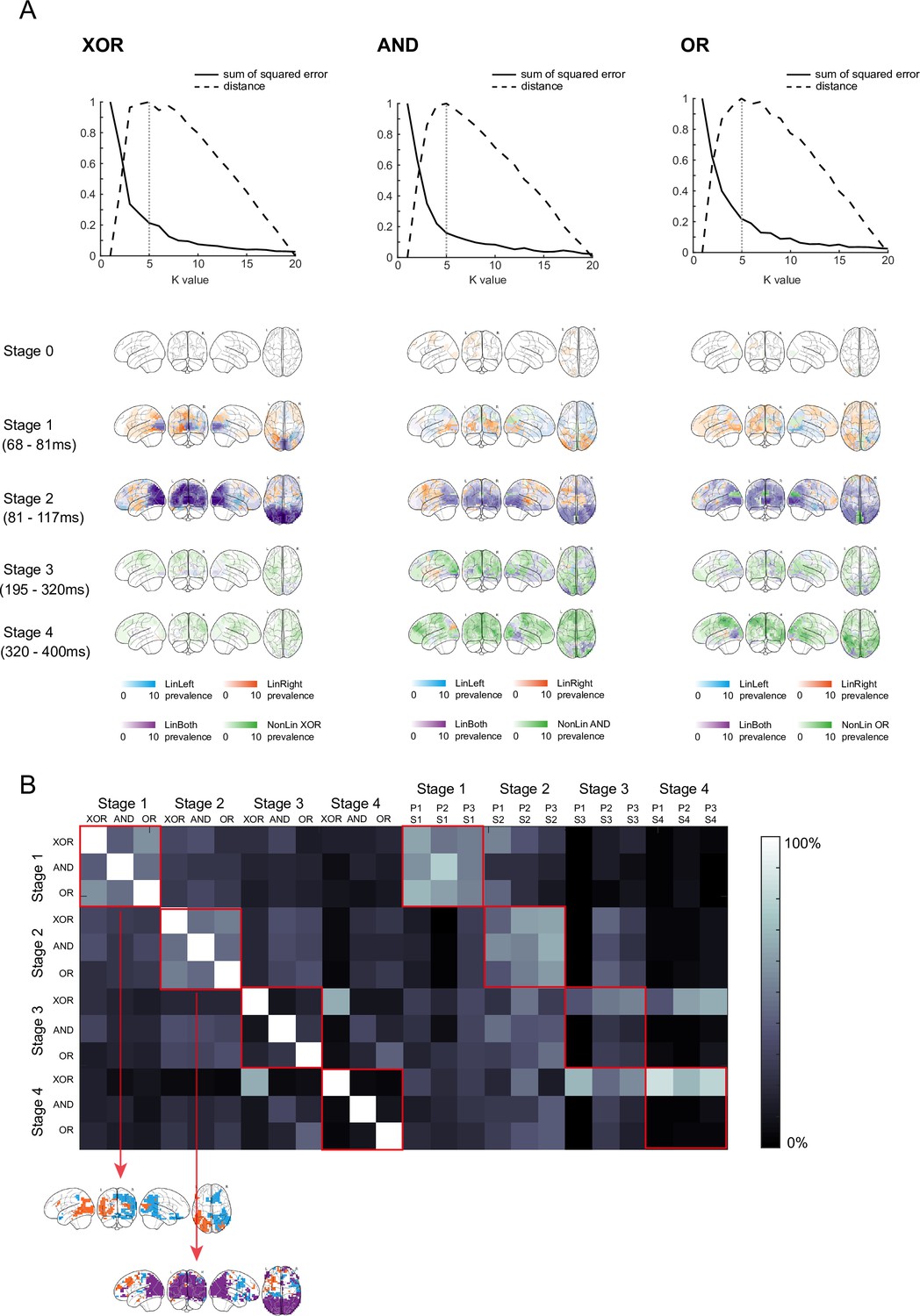
Clustering of computation stages.
(A) Number of computation stages. Results of k-means analysis, with k = 1...20, with sum of squared error of each k (plain curve) and distance of the plain curve from straightline (dashed curve). We selected the k with furthest distance (elbow method). At stage 0, there is no computation. At stage 1, LinLeft (blue) and LinRight (orange) dominate. At stage 2, LinBoth (magenta) dominates. At stages 3 and 4 the task-specific NonLin XOR, AND, and OR (green) dominate. Color intensity reflects the frequency of participants performing this computation in this stage and source. (B) Similarity of computation stages across XOR, AND, and OR. We computed pairwise similarities between the four computation stages of each task, as the percentage of sources that shared the same computation (either LinLeft, LinRight, BothLin, NonLin XOR, AND, or OR) across pairs of stages. Similarity is high between stages 1 and 2 across the three tasks (color-coded brains show the sources with intersecting computations across the three tasks), whereas the NonLin stages 3 and 4 are task specific. (C) Generalization of stages of computation in XOR from face to Gabor stimuli. Using the similarity metric again, we demonstrate the generalization of the three participants (P1, P2, P3) who resolved XOR with Gabor stimuli (Figure 1—figure supplement 3), showing similarity of their stages 1 and 2 with those of the face stimuli, and similarity of stages 3 and 4 only with the XOR face stage.
Figure 1—figure supplement 2
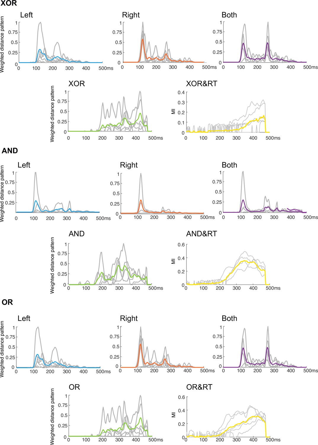
Results for individual participants.
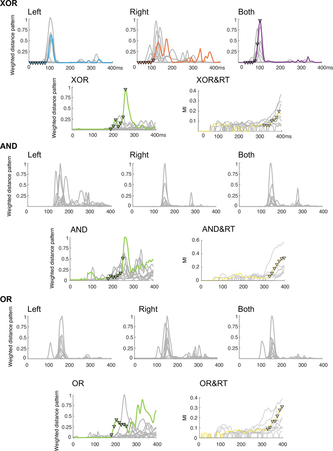
Gray curves correspond to the individual participants’ time courses of the individual source Lin (left and right), LinBoth, NonLin, and NonLin&RT, in the XOR, AND, and OR tasks. Only significant (familywise error rates p=0.05) time points are shown, other time points are set to 0. The colored lines correspond to the data of one exemplar participant used in Figure 3 (XOR) and 3 (AND and OR). Tick marks on each colored line correspond to the seven time-steps of the dynamic unfolding of each computation.
Figure 1—figure supplement 3
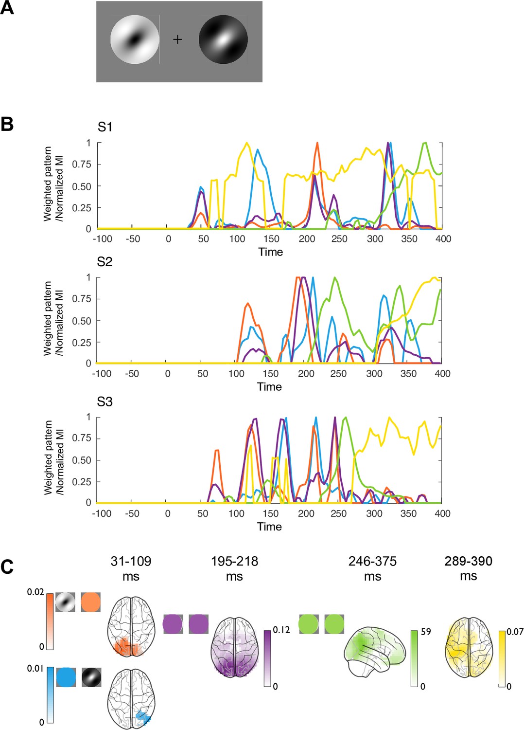
Replication of four stages of computation with Gabor stimuli.
(A) Stimuli. In three participants, we presented two spatially separated Gabor and phase-opposed Gabor patches. Participants responded when the two patches had the same vs. different colors with different keyboard keys (an XOR task). Gabors were presented in four randomly chosen orientations, spanning in total 11 × 11 deg of visual angle (the inner edges of each Gabor were located ~5.7 deg of visual angle away from the centrally presented fixation cross). Gabor inputs were simultaneously presented on the screen for 150ms. (B) Four hierarchical stages of computations. Each plot shows the maximum within participant of source-level (1) linear discrimination of each Gabor input Lin (blue and orange), (2) linear discrimination of both input, Linboth (magenta), (3) nonlinear integration of both inputs, NonLin (green) with the XOR task pattern, and (4) with amplitude variations that relate to reaction time (RT) NonLin&RT (yellow). (C) Colored brains localize the regions where these computations start. The brackets report the per participant onset times (for Lin, left and right) and peak latencies (for LinBoth, NonLin XOR, and XOR&RT), and averaged across participants in the colored brains.
Figure 1—video 1
Dynamic summary of the four stages of computation in the XOR task (data from the example XOR participant highlighted in Figure 1—figure supplement 2).
The left brain animation reports the voxel-level computations performed at each stage. Specifically, stage 1: LinLeft (light blue), LinRight (orange); stage 2: LinBoth (magenta); stage 3: NonLin XOR (green); stage 4: NonLin XOR&RT (yellow). The schematic network illustrates each stage as it unfolds over time, with left and right hemispheres represented as the left and right network nodes. Scatter plots represent each dynamic computation at each stage in the 2D space of magnetoencephalographic response of the source with highest metric for this computation. In the scatter, each color-coded dot represents the average source response to each one of the four classes of color-coded stimuli (see adjacent legend). The specific computation exerted on the same four classes of stimuli is provided in the discrimination line (or curve) in the legend. Note that the first two stages comprise only linear computations that represent the stimuli; the latter two comprise nonlinear computations that related to the specific task performed. Figures 1 and 2, and Figure 1—figure supplement 1B show that only the latter two nonlinear stages change with task (XOR, AND, and OR).
Figure 2 with 2 supplements
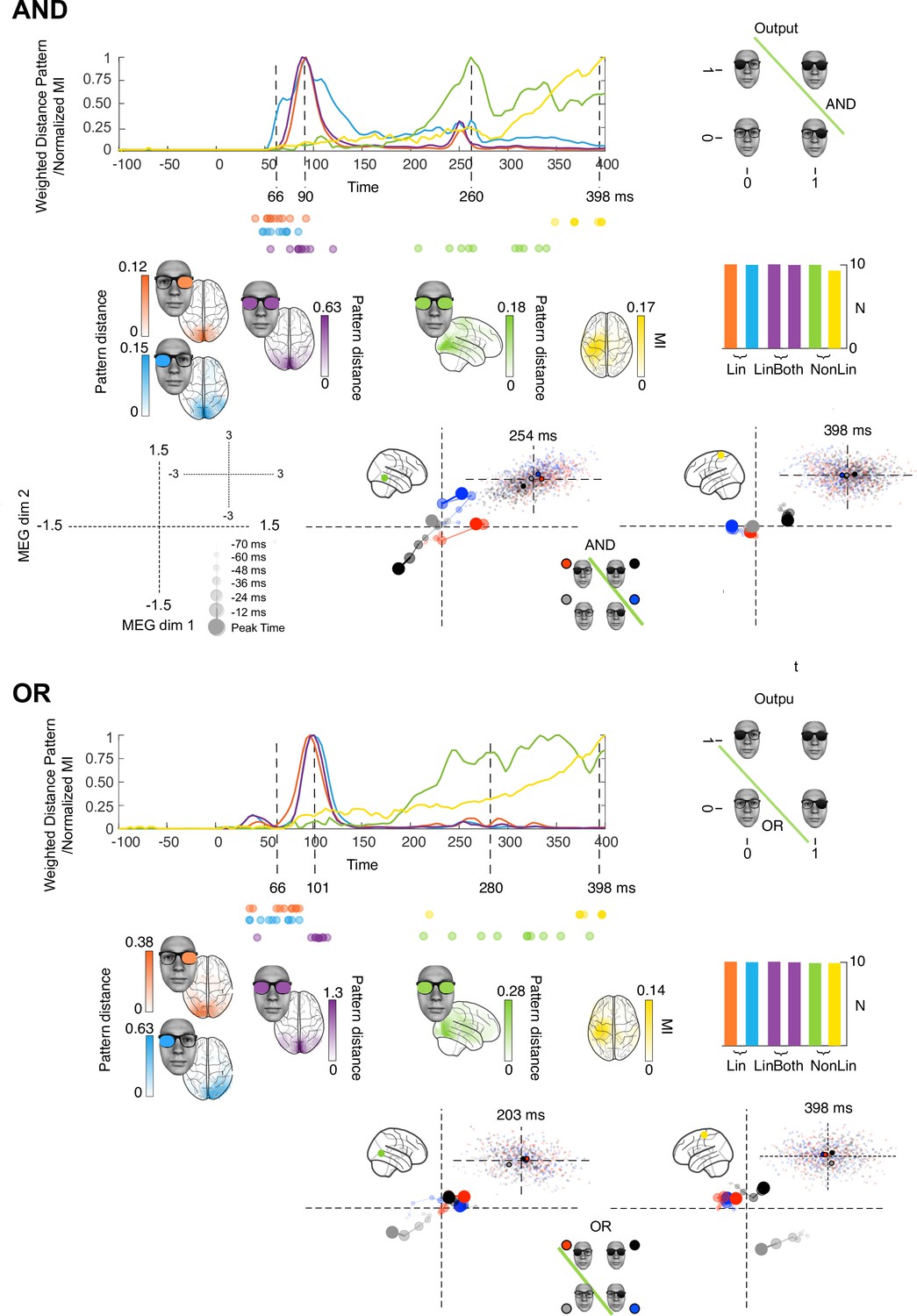
Stages of computations in AND and OR tasks.
Each colored curve averages (N = 10 participants) the time courses of the maximum across sources that: (1) linearly discriminates (weighted distance pattern) in its magnetoencephalographic activity the ‘on’ vs. ‘off’ state of the left (blue) and right (orange) inputs, (2) linearly discriminates both inputs (magenta), (3) nonlinearly integrates both inputs with the respective task pattern and (4) nonlinearly integrates both inputs with the respective task pattern and with amplitude variations that relates to reaction time (RT) (yellow). Colored brains localize the regions where these computations start (onset times for left and right) or peak (peak latencies for LinBoth, NonLin, and RT) p<0.05 familywise error rates corrected with a permutation test, see Methods, Linear vs. Nonlinear Representations; Representation Patterns. Dots report the onset time of computation (1) and (2), and the peak time of computation (3) and (4) in each participant. See Table 2 and Figure 1—figure supplement 2 for individual participant replication of each computation in the same brain regions and time windows. Single source plots in each task develop the data of one typical observer, where the green and yellow computations (cf. color-coded sources in the glass brain) differ between AND, OR, and XOR (see Figure 3 for caption).
Figure 2—figure supplement 1
Four stages of computations replicated with delayed stimulus presentation.
Using the same face stimuli as in the main experiment, we presented either the right or the left input as gray for the first 1000ms following stimulus onset. The other input was either clear or dark. After 1000ms, the gray input changed into either clear or dark. Participants waited until the gray input changed and then responded according to the logic gate task: XOR (N = 5, top), AND (N = 4, middle), and OR (N = 5, bottom) (two participants were excluded under the same criteria as the main experiment). Linear representation of the first input started around 80ms poststimulus (with a ~100ms peak; or around –900ms with respect to second lens presentation). The second input was linearly represented from ~100ms with a peak at ~120ms (blue, orange, and magenta time courses). Averaged time courses of the Lin and NonLin computations across individual participants (see Figure 2—figure supplement 2) replicated the results of Figure 1.
Figure 2—figure supplement 2
Four stages of computations replicated with delayed stimulus presentation: individual participants’ results.
Gray curves correspond to the individual participants’ time courses of the individual source Lin (left and right), LinBoth, NonLin, and NonLin&RT, in the XOR, AND, and OR tasks, with 0ms corresponding to the time point when the second input is revealed (i.e. when the gray lens turns clear or dark, Figure 2—figure supplement 1). The colored lines correspond to the mean across participants.
Figure 3 with 1 supplement

Dynamic unfolding of different computations on the same inputs (e.g. XOR participant, see also Figure 1—video 1 ).
(A) Localized sources. Color-coded source localized in the top glass brain illustrates each color-coded computations in each scatter plot. Legend. Axes of the scatter plots represent the 2D source magnetic field response. Small dots are single-trial source responses; larger dots their averages for each color-coded stimulus class, dynamically reported over seven timesteps (cf. legend) corresponding to the seven triangular markers in Figure 1—figure supplement 2, XOR. Increasing dot sizes, saturations, and connecting lines denote increasing timesteps of the dynamic trajectory. (B) Right occipital. The light blue discrimination line indicates the linear (LinLeft) computation that this source represents at the seventh timestep (cf. adjacent scatter for the distribution of individual trials at this time). Inset vector diagram provides a geometric interpretation of the linear computations. Using stimulus [0,0] as the origin: blue arrow illustrates source response to stimulus [0,1] (blue disk); red arrow shows source responses to [1,0] (red disk); gray disk illustrates linear summation of these vectors (opaque lines); black disk is the observed mean response to stimulus [1,1]. (C) Left occipital. Same caption for orange LinRight computation. (D) Right midline occipital and (E) right fusiform gyrus. Same caption for magenta LinBoth computation. (F) Right parietal and (G) postcentral gyrus. Same caption for green XOR nonlinear computations. Green vector shows discrepant nonlinear observed response to stimulus [1,1] and linear sum of responses to [0,1] and [1,0].
Figure 3—figure supplement 1
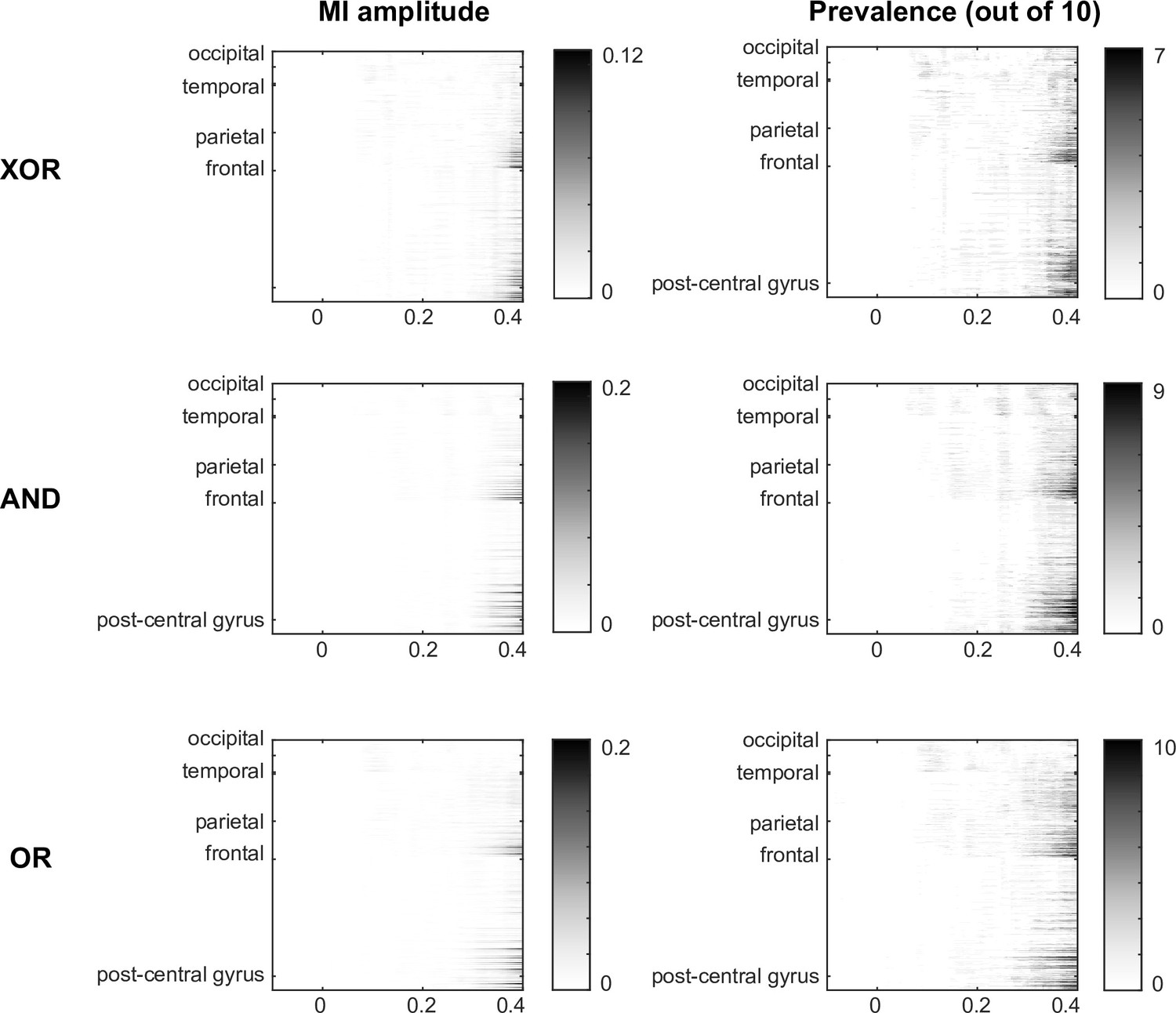
Dynamics of relation of magnetoencephalographic (MEG) responses to reaction times (RTs).
In each task, for each participant, we computed the single-trial relationship between variations of MEG source amplitude at each time point and RT, computed as mutual information (MI) (< RT; MEGt>). Left plots show the average of significant MI (p<0.05, corrected). Right plots show the number of participants with significant MI in each source and time point. In each task, stage 4 postcentral gyrus (and to some extent frontal regions) source activity relates to behavioral RTs.
Figure 4
Computation of representation patterns.
Note: the face stimulus was artificially synthesized and so does not belong to any real person.
Author response image 1
This image shows the changes to the main results presented in Figures 1 and 3 between the original and the revised manuscripts.
The color-coded curves present each computation. We can now better see the 4 distinct stages (cf. 4-stage image above), where the brief timing of Stage 1 (in orange and blue, LinLeft and LinRight computations) is now better decoupled from that of Stage 2 (in magenta, LinBoth). Individual participants peak time results for each computation (represented as colored dots) further demonstrates the decoupling into four stages.
Tables
Table 1
Mean behavioral accuracy and median reaction times in XOR, AND, and OR, 95% percentile bootstrap confidence interval shown in brackets.
All pairwise comparisons, p>0.05.
| Accuracy | Reaction time | |
|---|---|---|
| XOR | 98.5% [97, 99] | 499ms [461, 557] |
| AND | 99% [98.6, 99.5] | 457ms [393, 505] |
| OR | 99.3% [99.2, 99.5] | 490ms [439, 541] |
Table 2
Number of individual participant replications of the four color-coded computations, within the same region and time window.
Lin, left and right occipital sources [74–117ms]; LinBoth, occipital midline and right fusiform gyrus [74–117ms]; NonLin, XOR: parietal [261–273ms], AND: temporal-parietal [246–304ms], OR: temporal-parietal [261–304ms]; RT, postcentral gyrus [386–398ms]. Bayesian population prevalence (Ince et al., 2021) of 9/10 = 0.89 [0.61 0.99]; 10/10 = 1 [0.75 1] (MAP [95% HPDI]).
| Lin | LinBoth | NonLin | NonLin&RT | |
|---|---|---|---|---|
| XOR | 10/10 | 10/10 | 9/10 (parietal) | 9/10 |
| AND | 10/10 | 10/10 | 10/10 | 9/10 |
| OR | 10/10 | 10/10 | 10/10 | 10/10 |
Additional files
Download links
A two-part list of links to download the article, or parts of the article, in various formats.
Downloads (link to download the article as PDF)
Open citations (links to open the citations from this article in various online reference manager services)
Cite this article (links to download the citations from this article in formats compatible with various reference manager tools)
Different computations over the same inputs produce selective behavior in algorithmic brain networks
eLife 11:e73651.
https://doi.org/10.7554/eLife.73651


