Structure and function of axo-axonic inhibition
- Allen Institute for Brain Sciences, United States
- Princeton Neuroscience Institute, Princeton University, United States
- Computer Science Department, Princeton University, United States
- Brain & Cognitive Sciences Department, Massachusetts Institute of Technology, United States
- Department of Neuroscience, Baylor College of Medicine, United States
- Center for Neuroscience and Artificial Intelligence, Baylor College of Medicine, United States
- Department of Electrical and Computer Engineering, Rice University, United States
- Department of Neurology, University of British Columbia, Canada
Figures
Figure 1 with 4 supplements

A map of axon initial segment (AIS) input from electron microscopy (EM).
(A) A block of tissue was selected from L2/3 of mouse V1 and processed in an EM pipeline. (B) Serial 40 nm sections were imaged computationally aligned into a volume. (C) Image annotation pipeline. Left: images were taken with 3.58 × 3.58 nm pixels. Scale bar is 500 nm. Center: the neuropil was densely segmented and targeted proofreading was done to correct pyramidal neurons (PyCs) and other objects of interest. Right: automated synapse detection identified pre- and postsynaptic locations for synapses and was followed by targeted proofreading for false positives. To interactively view the dataset in 3D, visit https://www.microns-explorer.org/chc/soma/all_by_type. (D) For each PyC with significant AIS in the volume, we started with the overall morphology and synaptic inputs (cyan dots) and computationally extracted the AIS (dark gray) and its synaptic inputs (cyan arrows). All AIS bounds can be seen in 3D at https://www.microns-explorer.org/chc/soma/ais_bounds. (E) Soma, AIS, and AIS synaptic inputs for all PyC analyzed. The volume is rotated so that the average AIS direction is exactly downward. Note that dendrites and higher-order axon branches are omitted for clarity. (F) Histogram of synapses per AIS. Synapse data can be found in Supplementary file 2.
Figure 1—figure supplement 1
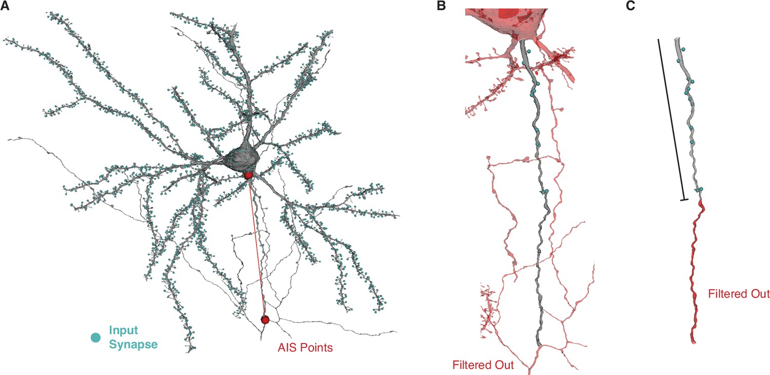
Axon initial segment (AIS) segmentation pipeline.
(A) In order to extract the AIS synapses from each pyramidal cell, we manually annotated the AIS bounds for each cell by placing one point at the structural base of the AIS and a lower point defined by the first branch point, myelination, or the edge of the image volume. Blue spheres indicate synaptic inputs. (B) We computationally extract the mesh and its associated synapses between the AIS bounds. (C) For Figures 3 and 4, we further filter out the AIS beyond an initial length (see Figure 3A). To interactively view all pyramidal neurons (PyCs) with AIS bounds in 3D, visit https://www.microns-explorer.org/chc/soma/ais_bounds.
Figure 1—figure supplement 2
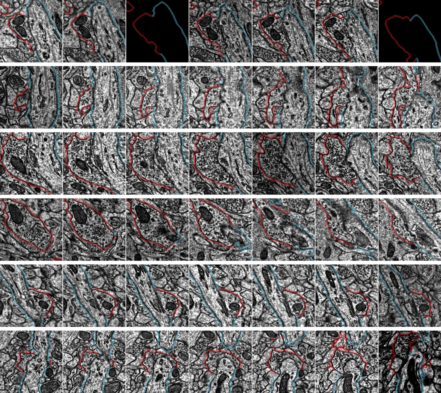
Example synapse imagery for all axon initial segment (AIS) inputs onto cell ID 648518346349535847.
Each row has seven serial sections with the center image centered on the synapse location from automated detection. The AIS is outlined in blue, the presynaptic axon is shown in red (if chandelier cell [ChC]) or purple (if non-ChC). Rows are ordered from the top of the AIS. Each panel is 1 µm × 1 µm. Some panels are black due to missing image data in certain sections. Input data for this AIS can be viewed in 3D at https://www.microns-explorer.org/chc/ais/28.
Figure 1—figure supplement 3
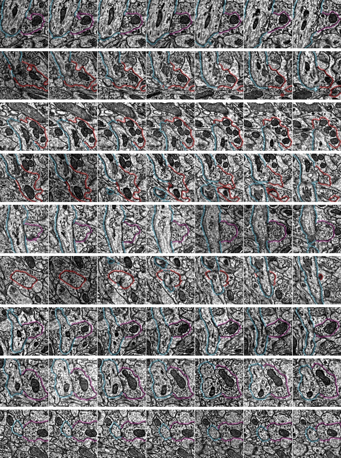
Example synapse imagery for all axon initial segment (AIS) inputs onto cell ID 648518346349539517.
Each row has seven serial sections with the center image centered on the synapse location from automated detection. The AIS is outlined in blue, the presynaptic axon is shown in red (if chandelier cell [ChC]) or purple (if non-ChC). Rows are ordered from the top of the AIS. Each panel is 1 µm × 1 µm. Some panels are black due to missing image data in certain sections. Input data for this AIS can be viewed in 3D at https://www.microns-explorer.org/chc/ais/112.
Figure 1—figure supplement 4
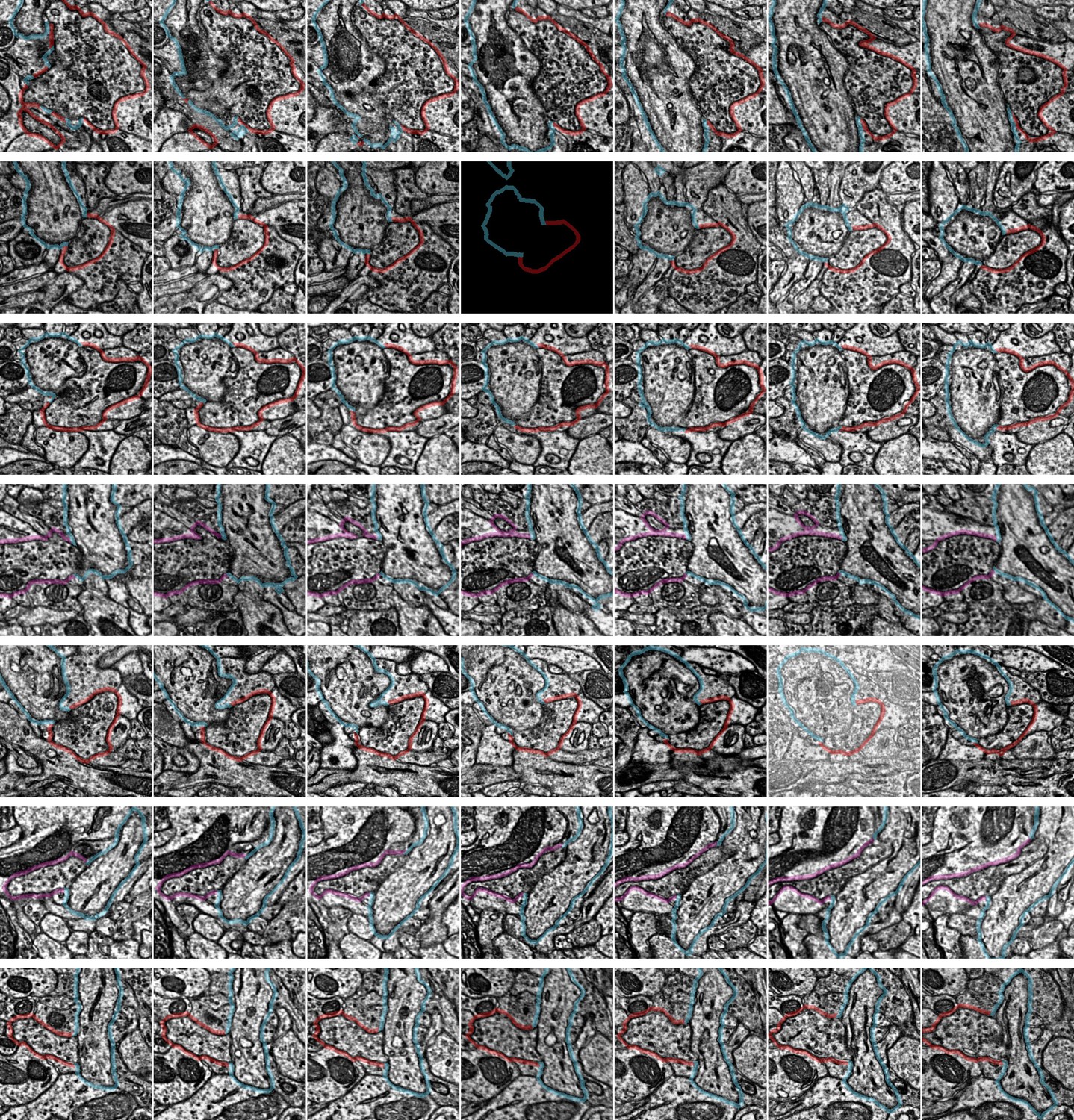
Example synapse imagery for all axon initial segment (AIS) inputs onto cell ID 648518346349539572.
Each row has seven serial sections with the center image centered on the synapse location from automated detection. The AIS is outlined in blue, the presynaptic axon is shown in red (if chandelier cell [ChC]) or purple (if non-ChC). Rows are ordered from the top of the AIS. Each panel is 1 µm × 1 µm. Some panels are black due to missing image data in certain sections. Input data for this AIS can be viewed in 3D at https://www.microns-explorer.org/chc/ais/115.
Figure 2 with 4 supplements
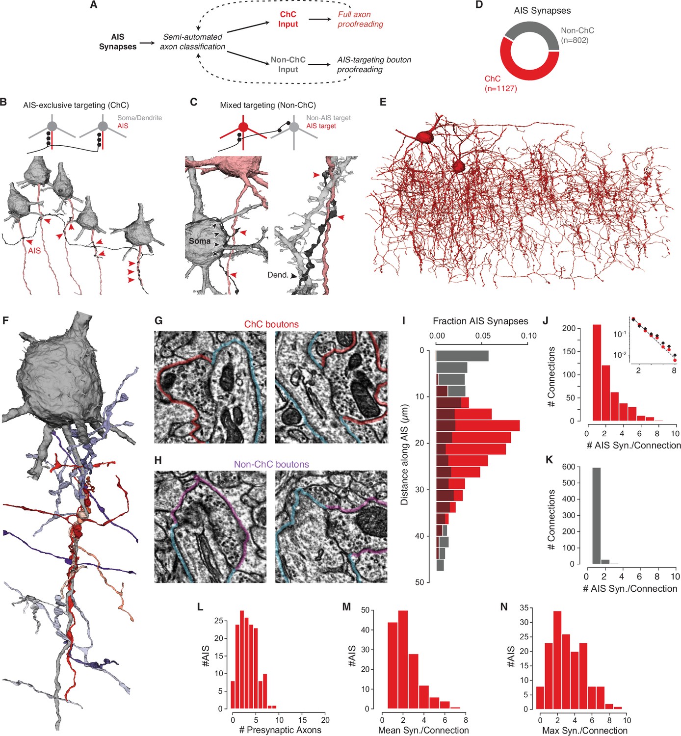
Characterization of axon initial segment (AIS) input.
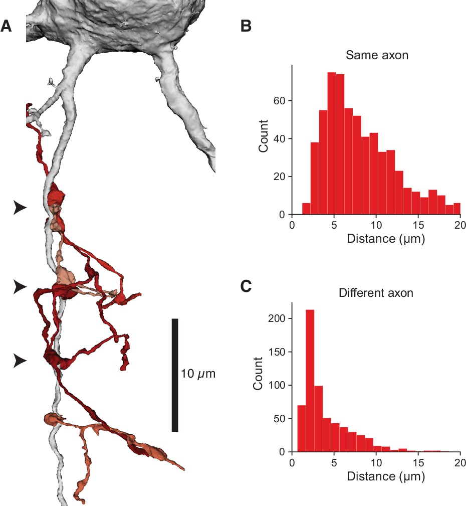
(A) Classification and proofreading workflow. Across AIS synaptic inputs, morphology and connectivity were used to distinguish chandelier cell (ChC) from non-ChC axons. ChCs were given full proofreading to get as-complete-as-possible arbors. For non-ChC inputs, all AIS-targeting boutons were proofread to ensure they were not due to merged-in ChC axons. The pipeline was repeated until no new axons were identified. (B) Axons that exclusively synapsed onto pyramidal neuron (PyC) AISes were classified as ChCs. Example below shows an axon targeting the AIS of several PyCs (red arrowheads). (C) Axons that showed mixed AIS and non-AIS targeting were classified as non-ChC. Example at left shows an axon (black) targeting an AIS (red arrowheads) and a nearby soma (black arrowheads). Example at right shows an axon (black) targeting a dendrite (black arrowheads) and an AIS (red arrowheads). (E) All ChC objects identified from the AIS survey. (F) Single PyC soma and AIS shown with presynaptic axons. Reds indicate ChCs, purples indicate non-ChCs. Axons are truncated to the region near AIS contacts for clarity. For the full data in 3D, please visit https://www.microns-explorer.org/chc/ais/80. (G) Example ChC synapse imagery for the AIS in (F). The AIS outlined in blue, ChC bouton in red. Image panels are 1 µm × 1 µm. (H) Example non-ChC synapse imagery onto the AIS in (F). As in (G) but with purple outlines for boutons. (I) Histogram of distance from AIS base for ChC (red) and non-ChC (gray) synapses. (J) Distribution of AIS synapses per connection for ChCs. Inset: semilog-y synapses per connection for all ChCs (red dots) and only ChC axon fragments with more than 20 synapses (black dots), with Poisson fit to the complete data (dashed line). (K) Distribution of AIS synapses per connection for non-ChCs. (L) Number of distinct presynaptic ChC axons per AIS. (M) Distribution of mean number of synapses in a ChC connection for each AIS. (N) Distribution of the number of synapses in the most numerous ChC connection on each AIS. Synapse data can be found in Supplementary file 2.
Figure 2—figure supplement 1
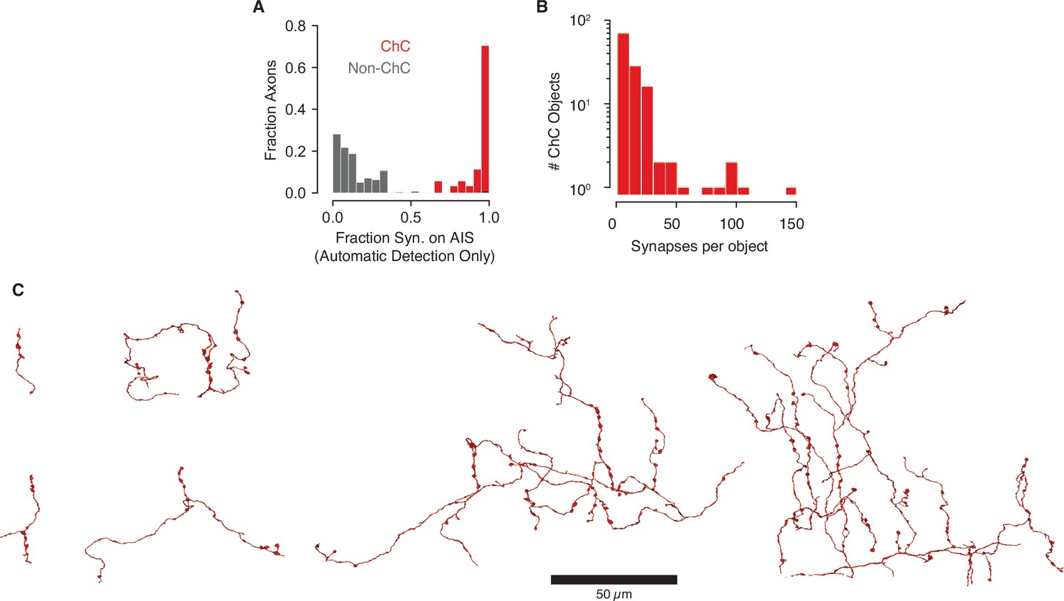
Characterization of orphan axons.
(A) Fraction of all automatically detected synaptic outputs that are onto the axon initial segment (AIS) (as opposed to soma or dendrites) from AIS-targeting axons onto the 153 core pyramidal neurons (PyCs). Chandelier cells (ChCs) shown in red, non-ChCs in gray. Only axons with three or more synapse are shown for clarity. Non-AIS synapses from ChCs were subsequently proofread (see main text). (B) Distribution of the number of synapses per ChC axon, including targets outside the 153 core PyCs. (C) Example morphologies of orphan ChC axon fragments. All ChC axons can be viewed online at https://www.microns-explorer.org/chc/axon/all_chc.
Figure 2—figure supplement 2
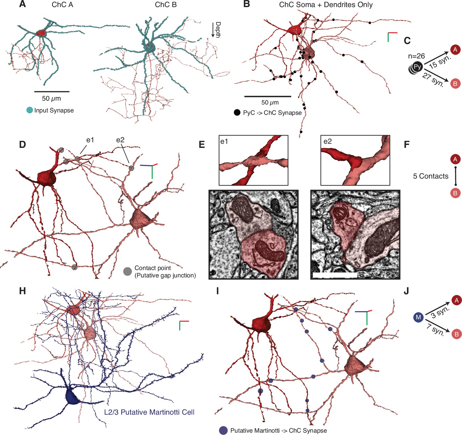
Examples of chandelier cell (ChC) dendrites and dendritic input.
(A) We found two clear ChCs with significant dendritic processes and synaptic inputs (blue dots) in the volume, which we label as ChC A and ChC B for this figure. Examples are shown individually. (B) Identified pyramidal neurons (PyCs) within the volume formed synapses onto the two ChCs (black dots). ChCs are shown in their observed locations. (C) Breakdown of connections: 26 PyCs in total made 15 synapses onto ChC A and 27 onto ChC B. (D) We observed five sites of dendrodendritic contacts with ultrastructural densities (gray dots). (E) Zoomed view of two example contacts (3D above, imagery below) indicated in (D) as e1 and e2. (F) Network breakdown of observed contacts. (H) The two ChCs received input from the single putative L2/3 Martinotti cell in the dataset, as defined by characteristic spiny dendrites and surface-projecting axon. (I) Synapses from the putative Martinotti cell were distributed across the ChC dendrites (blue dots). (J) Network breakdown of the putative Martinotti connections. For plots (B, D, H, I), the view is indicated by axes where green indicates depth, red is along the positive x-axis, and blue is along the positive z-axis. Axis lines are 10 µm in length.
Figure 2—figure supplement 3
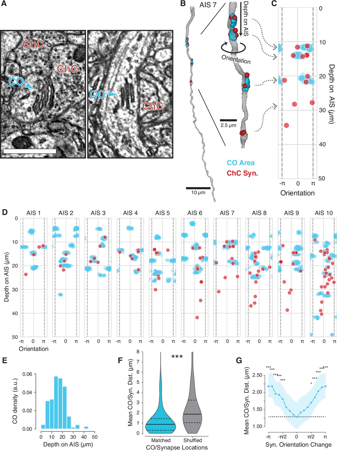
Chandelier cell (ChC) input is located near cisternal organelles (CO) on the axon initial segment (AIS).
(A) COs are stacked ER structures and clearly visible in electron microscopy (EM). (B) We identified the location of each CO (cyan clouds) and mapped it relative to ChC synaptic inputs (red dots). For each CO location and synapse, we measure its depth from the top of the AIS and the orientation around the AIS. Vertical gray dashed lines indicate where the orientation value wraps over. (C) Depth vs. orientation (in radians) plot for the AIS shown in (B). (D) Depth vs. orientation plots for all AIS with labeled COs. (E) Depth distribution of COs on the AIS. (F) Distribution of the distance between ChC synapses and the nearest CO along the surface (Matched) and the condition where synapses (but not COs) were remapped to the same depth and orientation on a different AIS (Shuffled). Black lines indicate median, dashed lines are interquartile interval. (G) Distance between a ChC synapse and the nearest CO when synapses were rotated in orientation along the same AIS. The dashed line is the value with no rotation. Dots indicate median, shaded region is the interquartile interval. In (F) and (G), comparison is by t-test. *p<0.05, **p<0.01, ***p<0.001.
Figure 2—figure supplement 4
Clusters of chandelier cell (ChC) inputs on the axon initial segment (AIS).
(A) Example AIS with multiple presynaptic ChC axons (reds) forming boutons in three distinct clusters (arrowheads). One additional synapse is below. (B) Distribution of distances from each ChC synapse to its nearest synapse from the same ChC axon. (C) Distribution of distances from each ChC synapse to its nearest other ChC axon.
Figure 3 with 3 supplements
Structural properties associated with chandelier cell (ChC) synaptic input.
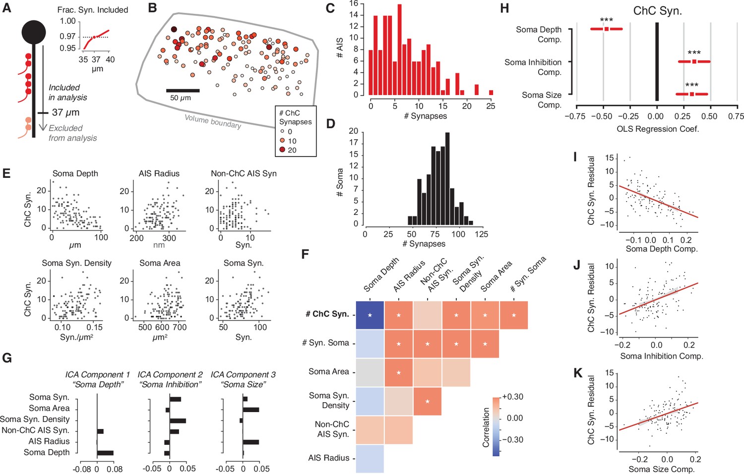
(A) For each axon initial segment (AIS), we look only at synapses on the first 37 µm, which captures 97% of all ChC synapses while omitting as few cells as possible from analysis. (B) Soma location for cells with complete soma in the volume, colored by total ChC synapse count. Pia direction is up. (C) Distribution of total ChC synapse count across pyramidal neurons (PyCs). (D) Distribution of total somatic synapses across PyCs. (E) ChC synapse count vs. six structural properties of soma and AISes: depth, AIS radius, non-ChC AIS synapse count, soma synapse density, soma area, and soma synapse count. (F) Pearson correlation matrix between all structural properties. Entries with an asterisk are significant (p<0.05) after Holm–Sidak multiple test correction. (G) Independent components analysis (ICA) components for PyC structural properties. Components are oriented so that the highest loading element is positive. Each component is labeled with an approximate interpretation of its combination of properties. (H) Standardized ordinary least-squares (OLS) regression coefficients for ChC vs. the three ICA components. Bars indicate 95% confidence interval; stars indicate significance after Holm–Sidak multiple test correction. ***p<0.001. (I) Scatterplot and linear fit of residual ChC synapse count vs. depth after fitting the other two components. Shaded region indicates the 95% confidence interval estimated from bootstrap (N = 1000). (J) Same as (I), but for the soma inhibition component. (K) Same as (I), but for soma size component. Synapse and AIS data can be found in Supplementary file 2.
Figure 3—figure supplement 1
Soma synapse labeling and measurements.
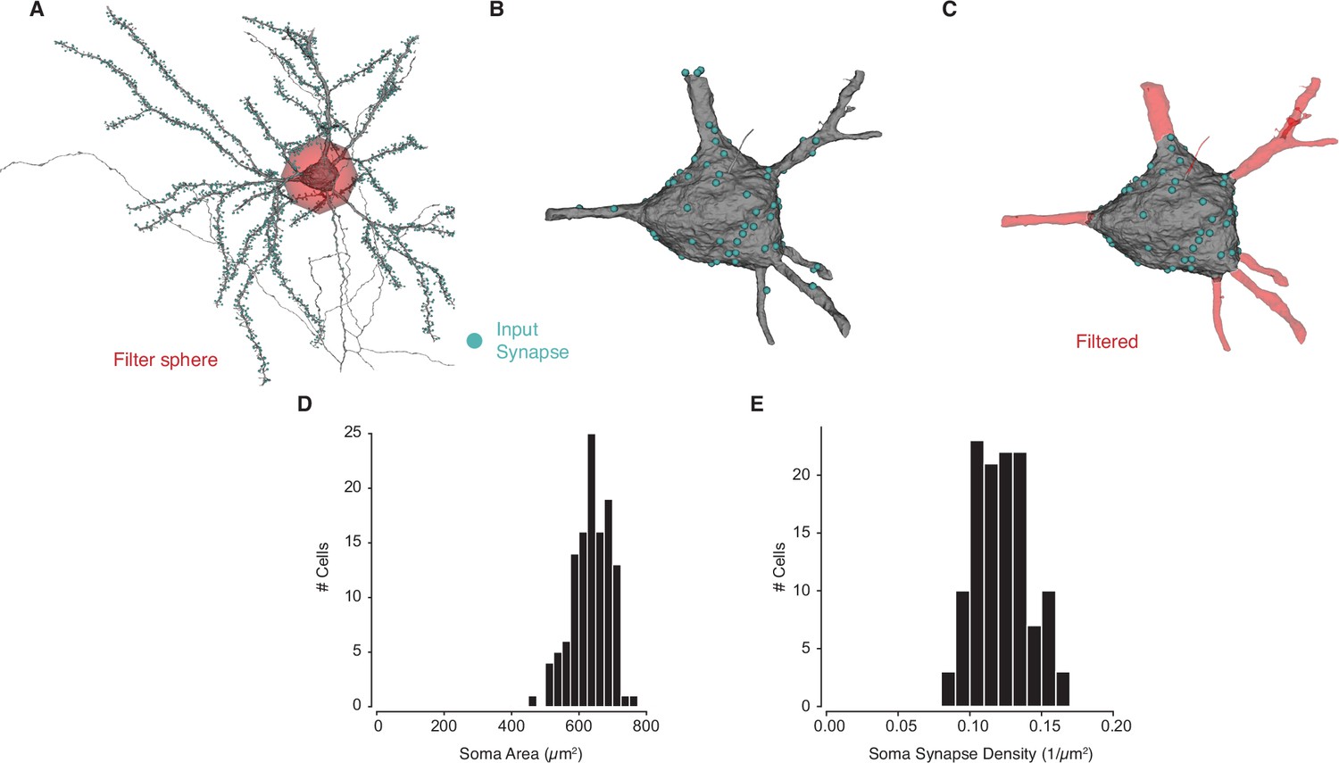
(A) For each pyramidal neuron (PyC), we filtered out a 30 µm ball around the center of each cell body. (B) The part of the mesh within this ball contains both soma and proximal dendrites. (C) To extract the soma alone, we filter out dendrites based on abrupt changes in radius, leaving a soma mesh and associated synapses. (D) Measured surface area for PyCs with soma in the volume. (E) Soma synapse density for PyCs with soma in the volume.
Figure 3—figure supplement 2
Distribution of synapses in the volume.
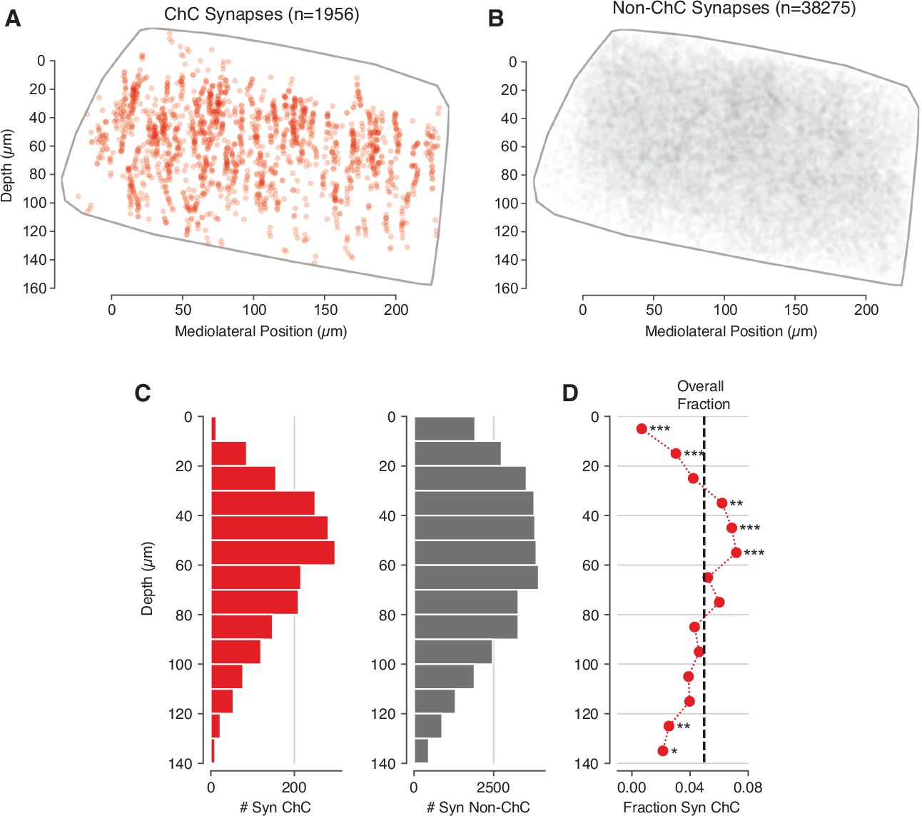
(A) Location of all synapses from chandelier cell (ChC) axons in the volume, whether onto pyramidal neurons (PyCs) in the analysis set or not. (B) Location of all synapses from non-ChC axon initial segment (AIS)-targeting axons. Note that this can include false merges. (C) Distribution of ChC and non-ChC synapses with depth. (D) Fraction of all synapses from AIS-targeting axons at a given depth that are from ChCs. Dashed line indicates the ChC synapses across all depths within L2/3. Stars indicate a significant difference from the L2/3 average from Fisher’s exact test after Holm–Sidak multiple test correction. *p<0.05, **p<0.01, ***p<0.001.
Figure 3—figure supplement 3

Scatterplots of pyramidal neuron (PyC) structural independent components analysis (ICA) components.
Lines indicate linear fit, shaded region indicates 95% confidence interval estimated from bootstrap. (A) Soma inhibition vs. soma depth components. (B) Soma size vs. soma depth component. (C) Soma size vs. soma inhibition components.
Figure 4 with 1 supplement
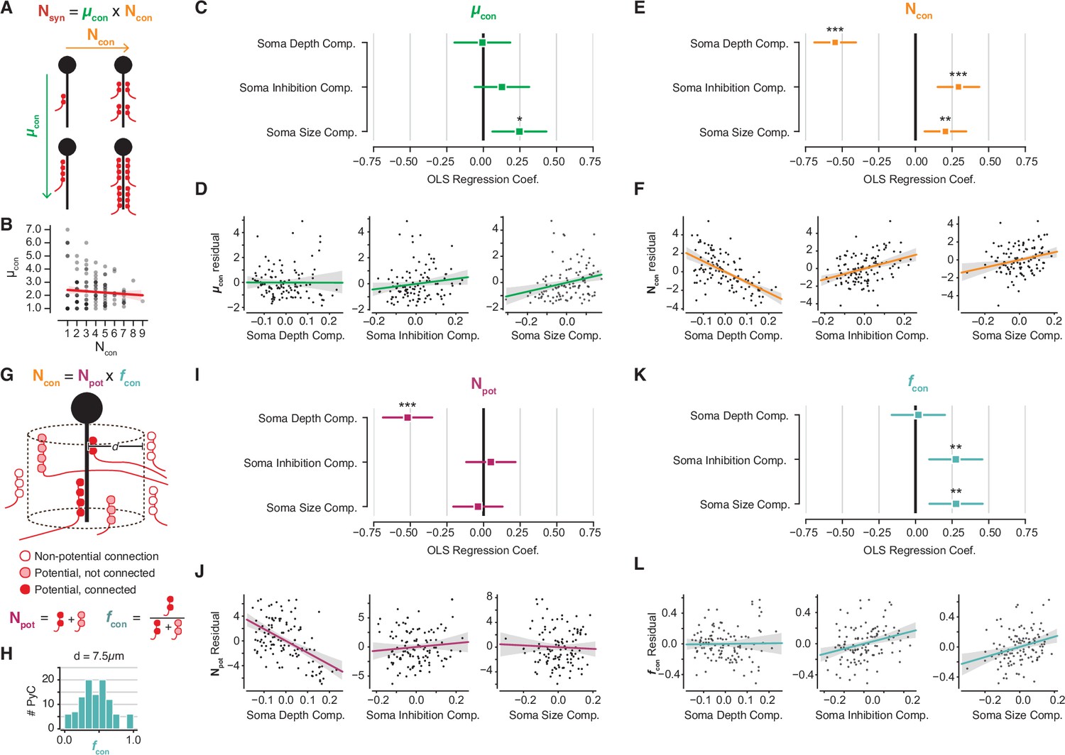
Decomposition of chandelier cell (ChC) synaptic input into constituent aspects.
(A) Synapse count can be broken into mean synapses per connection (µcon) times number of connections (Ncon). (B) Scatterplot of mean synapses per connection vs. number of connections for pyramidal neurons (PyCs) with soma in the volume. Red line indicates linear fit. (C) Standardized ordinary least-squares (OLS) coefficients for mean synapses per connection vs. independent components analysis (ICA) components, bars indicate 95% confidence interval. (D) Residual scatterplots of each ICA component vs. mean synapses per connection, as in Figure 3H–J. (E) Standardized OLS coefficients for number of connections. (F) Residual scatterplots for number of connections. (G) Number of connections can be broken into the number of potential connections (Npot) near an axon initial segment (AIS) times the fraction of those potential connections that form actual synapses (fcon). (H) Distribution of fcon for a potential radius of 7.5 µm, the value used for panels (I–L). Note that values span from 0 to 1. (I) Standardized OLS coefficients for potential connections. (J) Residual scatterplots for each ICA component vs. potential connections. (K) Standardized OLS coefficients for connectivity fraction. (L) Residual scatterplots for each ICA component for connectivity fraction. In all panels, stars indicate significance after Holm–Sidak multiple test correction. *p<0.05, **p<0.01, ***p<0.001.
Figure 4—figure supplement 1
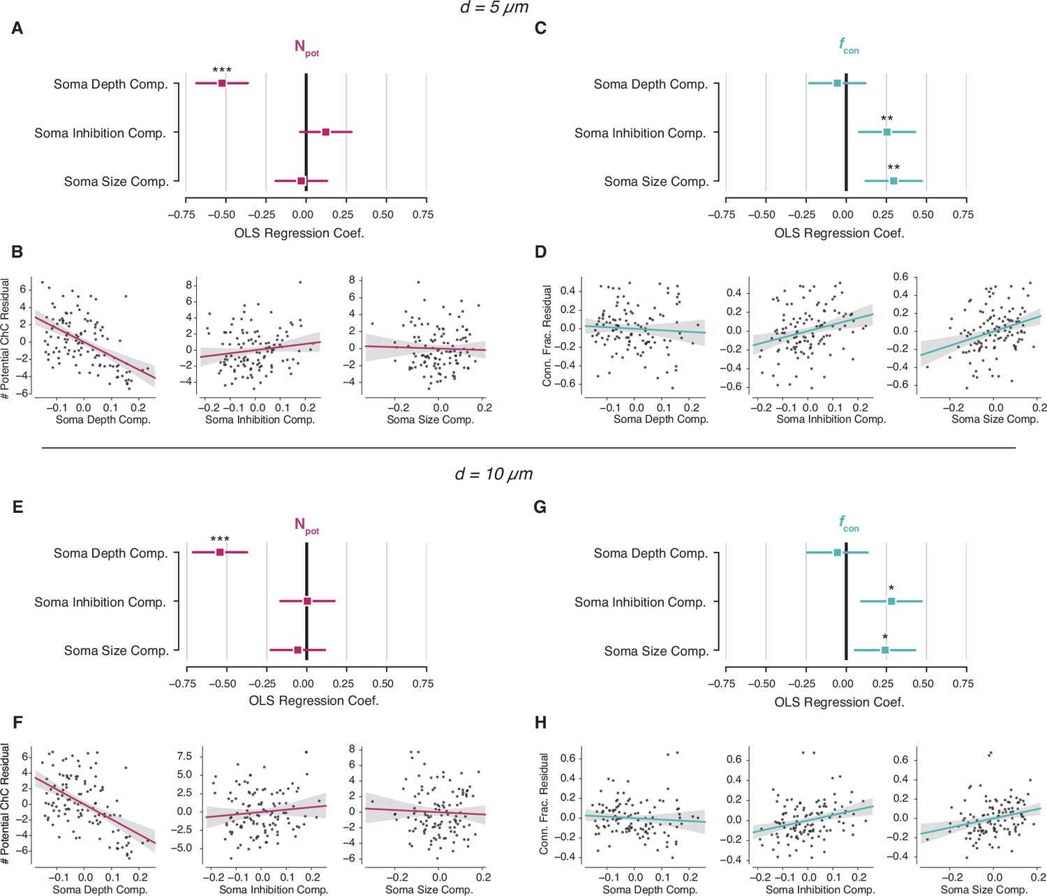
Potential connectivity analysis for other potential distance radii.
(A–D) Potential synapse analysis with a radius of 5 µm. (A) Standardized ordinary least-squares (OLS) coefficients for number of potential connections. (B) Residual scatter plots for number of potential connections. (C) Standardized OLS coefficients for connectivity fraction. (D) Residual scatterplots for connectivity fraction. (E–H) Same as (A–D), but for a connectivity radius of 10 µm. In all panels, stars indicate significance after Holm–Sidak multiple test correction. *p<0.05, **p<0.01, ***p<0.001.
Figure 5
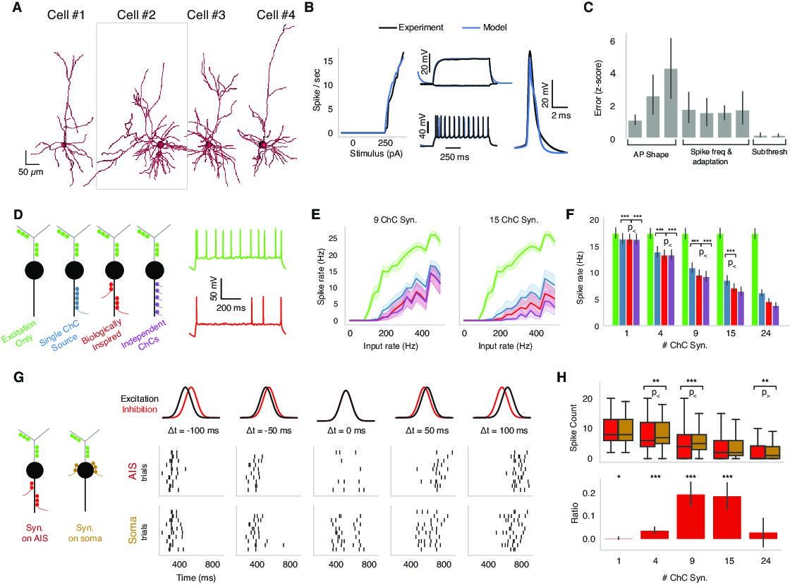
Biophysical modeling of chandelier cell (ChC) inhibition.
(A) Reconstructed morphologies for four pyramidal neurons (PyCs) from mouse V1. (B) Biophysically detailed, ion-conductance models were fit for each cell constrained by its slice electrophysiology features and reconstructed morphology. Panels show model response vs. experimental data for one case (cell #2 in panel A). The panel shows the model performance in terms of f-I-response, spike waveform similarity and example subthreshold, suprathreshold somatic voltage traces (black) vs. the actual experimental traces (blue). (C) Average z-scored training errors for the four models (cell #1–4) for a set of electrophysiology parameters. (D) Left: schematic for different ChC configurations (green: dendritic excitation; colors along axon initial segment [AIS]: ChC inhibition innervation). Three inhibitory innervation patterns are considered that affect the temporal aspect of ChC synapse activation. Right: intracellular voltage response at soma when only excitation is active (green) vs. when AIS inhibition is co-active (red). (E) Increasing excitatory synaptic drive vs. PyC spike rate for the different inhibition scenarios (colors) for 9 vs. 15 total ChC synapses along the AIS. Results from one cell model (cell #2 in panel A) for different innervation realizations (line: mean; shaded area: SD). (F) Average PyC firing rate across the four single-cell models at fixed excitation across ChC configurations for increasing number of ChC synapses (bar: mean; error bar: SD; significance testing: Wilcoxon signed-rank test at 5% false discovery rate). (G) Effect of AIS vs. somatic inhibition barrages on PyC spike output (black: excitatory input barrage; red: inhibitory AIS barrage; left-to-right: difference between centroids is −100, –50, 0, 50, and 100 ms, respectively). Raster plots: spike output for AIS (top) vs. somatic (bottom) inhibitory barrage (all other properties remain identical). When the two barrages are coincident, AIS inhibition results in a decrease in PyC spiking vs. somatic inhibition. Data shown for multiple realizations in one model (cell #2 in panel A). (H, top) PyC spike output count for inhibition at the AIS vs. at the soma across four models and multiple realizations. (Bottom) The differential effect in inhibition as computed by the difference between soma and AIS spike counts divided by the sum of the spike counts. The ratio ranges between –1 and 1, where 1 represents inhibition at the AIS being 100% more effective than at the soma and 0 meaning no differential effect. The most prominent difference between AIS and somatic inhibition is for concurrent barrages when the number of ChC synapses along the AIS is between 4 and 15. Significance testing: Wilcoxon signed-rank test at 5% false discovery rate.
Figure 6 with 1 supplement
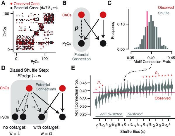
Geometrically constrained co-targeting motif analysis.
(A) Connectivity matrix from chandelier cell (ChC) axons onto pyramidal neuron (PyC) targets. Each black dot represents one potential connection for a distance threshold of 7.5 µm, and each red dot represents one actual connection with any number of synapses. Elements are clustered by the potential connectivity matrix, suggesting that most of the structure of the network comes from geometry alone. (B) Cartoon of a potential bifan motif. In a bifan motif, two ChCs would target the same pair of PyCs. In a potential bifan motif, three of those connections are present and the fourth is a potential connection. We consider the probability p that this potential edge is connected. (C) Observed connectivity probability for the potential bifan motif in our dataset (red line) compared to shuffled networks that preserve PyC in-degree and potential connectivity. We see no evidence of excess clustering of ChC targets beyond geometry. (D) Cartoon of a biased bifan shuffle, where potential connections that complete a bifan motif are given a different weight in the shuffle probability. Setting the bias weight ɑ > 1 encourages co-targeting by ChCs, while setting the bias weight ɑ < 1 reduces co-targeting. (E) Observed connectivity (red line) probability vs. shuffled networks with different bias weights based on the shuffle step shown in (D) (gray violin plots, N = 1000 per bias weight value). Red stars indicate bias weights where the observed value is above (p>) or below (p>) 95% of the shuffled distribution. Even with the geometric constraints, we can rule out strong clustering or anticlustering within the data.
Figure 6—figure supplement 1
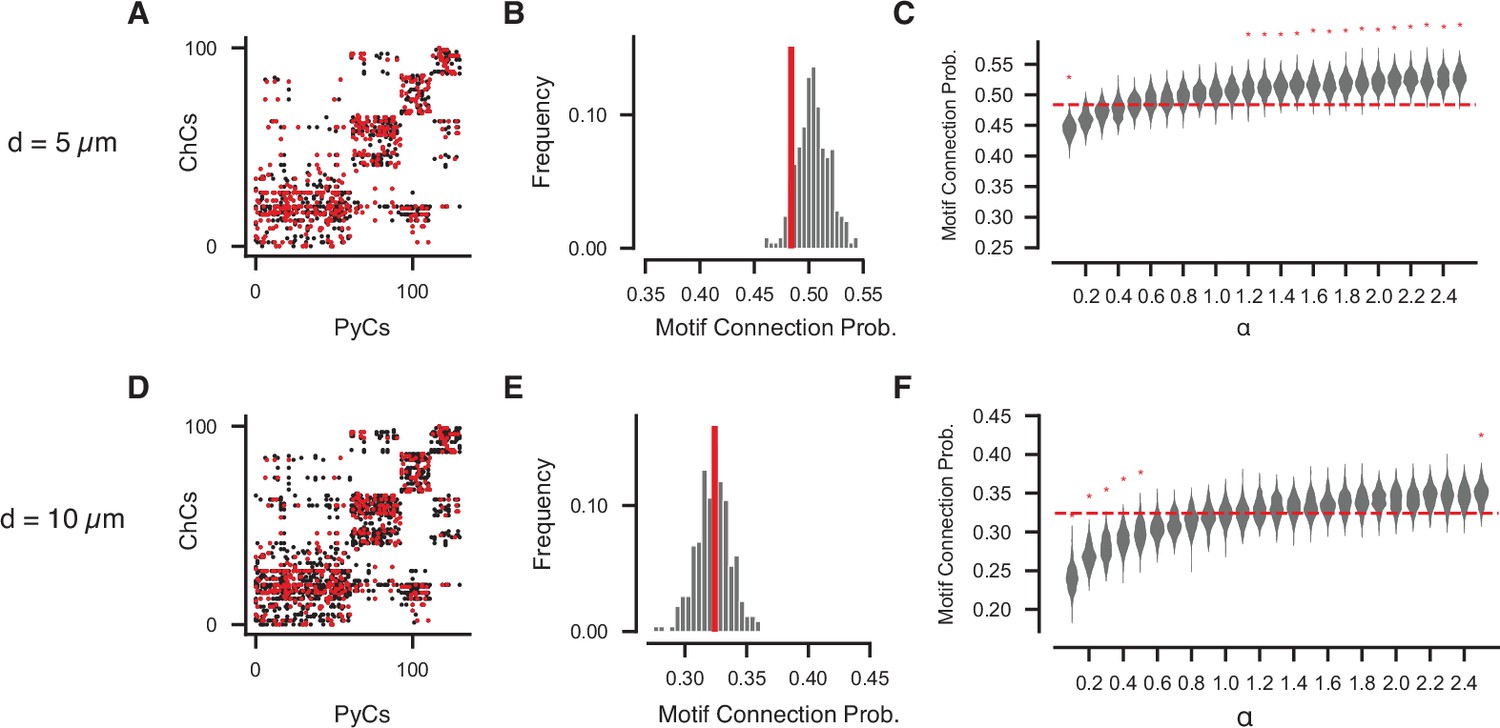
Geometrically constrained co-targeting motif analysis for other potential distance radii.
(A–C) Analysis for potential radius of 5 µm. (A) Potential (black) and actual (red) connectivity matrix, clustering shown on potential connectivity alone. (B) Observed connectivity probability for the potential bifan motif compared to shuffled networks that preserve pyramidal neuron (PyC) in-degree and potential connectivity (N = 1000 shuffled networks). Red line indicates observed value. (C) Potential bifan connectivity probabilities for networks with a shuffle bias, as in Figure 5E. (D–F) As in (A–C), but for a potential connectivity radius of 10 µm.
Figure 7
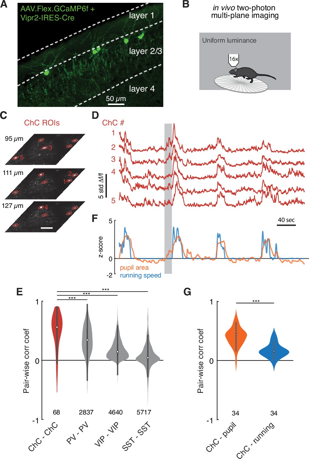
Functional imaging of chandelier cells (ChCs) reveals a synchronous response to arousal state.
(A) Maximum projection image in upper layers of V1 showing ChC-specific GCaMP6f expression in Vipr2-IRES2-Cre mice injected with AAV-Flex-GCaMP6f. Note cell bodies at the L1/L2 border, characteristic cartridges, and L1 dendrites. (B) Cartoon of experimental design. Mice expressing GCaMP6f in V1 ChCs were placed on a treadmill and imaged with multiplane two-photon microscopy while subject to a uniform luminance visual stimulus. (C) An experiment with simultaneous three-plane imaging (depth shown on left) with five distinct ChC regions of interest (ROIs), each measured from its best plane. Scale bar is 50 µm. (D) GCaMP6f responses (z-scored from baseline) for the same five ROIs as in (C). Note extremely correlated large events. (E) Simultaneous behavioral measurements for the same experiment as in (D). Increased pupil size, a measure of arousal state, and running bouts correspond to periods of high ChC activity. Note that there are periods where ChC activity and pupil area increase in the absence of running (e.g., the period noted by the gray box). (F) Pairwise Pearson correlation for spontaneous activity traces for different interneuron classes. ChCs measured from two imaging sessions each for three mice show high spontaneous correlation compared to other classes of interneurons as computed from comparable observations in the public Allen Institute Brain Observatory data. Number of distinct pairs is shown. (G) Pairwise correlations between ChC activity traces and behavioral traces show that ChCs are significantly more correlated with pupil area than with running. Number of distinct pairs is shown. Statistical significance for cell-cell correlations was computed with the Mann–Whitney U test, while for matched cell-behavior correlations significance was computed with the Wilcoxon signed-rank test. ***p<0.001.
Figure 8
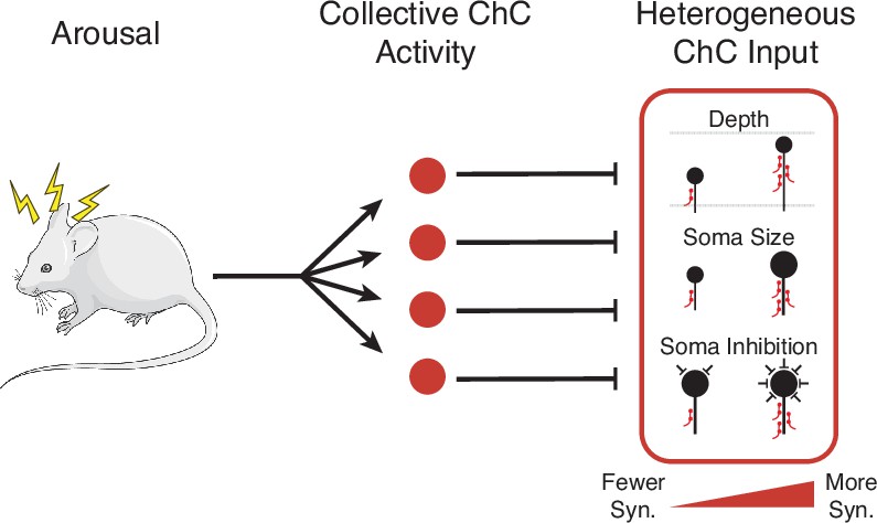
Cartoon summary of main results.
Arousal drives collective activation of chandelier cells (ChCs) in visual cortex.This common signal is passed into pyramidal neurons (PyCs) in a heterogeneous manner, with input onto each target cell modulated by cell-specific structural properties.
Videos
Video 1
A rendering of the electron microscopy (EM) reconstructions from this dataset demonstrating the mapping of chandelier cell (ChC) inputs onto layer 2/3 pyramidal neurons (PyCs).
Video begins with four gray PyCs with only their somatic regions and axon initial segment (AIS) region shown. An individual pink ChC fragment is slowly revealed over time as the reconstruction is followed along to all the locations that it synapses onto. Note that the portions of that axon that are far from the four PyCs are excluded from the rendering for clarity. Then a second, purple axon fragment is revealed in the same fashion. Third, all the ChC fragments that synapse onto these four PyCs are revealed simultaneously, each with their unique color. Finally, the scene reveals all the PyCs in this structural dataset, and all the ChC branches reconstructed in the dataset are revealed in red.
Tables
Key resources table
| Reagent type (species) or resource | Designation | Source or reference | Identifiers | Additional information |
|---|---|---|---|---|
| Antibody | Anti-GFP (chicken polyclonal) | Abcam | Cat# Ab13970; RRID:AB_300798 | (1:5000) |
| Antibody | Alexa-488 conjugated (donkey anti-chicken polyclonal) | Jackson ImmunoResearch | Cat# 703-545-155; RRID:AB_2340375 | (1:500) |
| Transfected construct (Mus musculus) | AAV1-CAG-FLEX-GCaMP6f | Addgene | Plasmid # 100835-AAV1; RRID:Addgene_100835 | Chen et al., 2013Used for ChC imaging |
| Transfected construct (M. musculus) | AAV5-CAG-FLEX-GCaMP6f | Addgene | Plasmid # 100835-AAV5; RRID:Addgene_100835 | Chen et al., 2013Used for ChC imaging |
| Transfected construct (M. musculus) | AAV9-CAG-FLEX-eGFP | Addgene | Plasmid # 51502-AAV9; RRID:Addgene_51502 | Oh et al., 2014Used for ChC imaging |
| Strain, strain background (M. musculus) | AI93 | The Jackson Lab | JAX Stock No. 024103; RRID:IMSR_JAX:024103 | Madisen et al., 2015Used for EM mouse |
| Strain, strain background (M. musculus) | Mouse: CamK2a-tTA/CamK2-Cre | The Jackson Laboratory | JAX Stock No. 003010; RRID:IMSR_JAX:003010 | Mayford et al., 1996Used for EM mouse |
| Strain, strain background (M. musculus) | Mouse: Vipr2-IRES2-Cre | The Jackson Laboratory | JAX Stock No. 031332; RRID:IMSR_JAX:031332 | Daigle et al., 2018Used for ChC imaging |
| Software, algorithm | Morphological and synapse analysis | This paper | https://github.com/AllenInstitute/ChandelierL23 (copy archived at swh:1:rev:f0087571f613eadf68cd6de0f93525a7ea949873, Schneider-Mizell, 2021) | |
| Software, algorithm | Eye tracking | Zhuang et al., 2017a, Zhuang, 2019 | https://github.com/zhuangjun1981/eyetracker | Version 3.1; Used for ChC imaging |
| Software, algorithm | Two photo image preprocessing | Zhuang et al., 2017a, Zhuang, 2017b | https://github.com/zhuangjun1981/stia/tree/master/stia | Used for ChC imaging |
| Software, algorithm | Brain Modelling Toolkit | Gratiy et al., 2018 | https://github.com/AllenInstitute/bmtk | Version 0.0.7. Used for whole-cell modeling |
Additional files
-
Supplementary file 1
A .csv file with a list of links to interactively explore the electron microscopy (EM) data and segmentation in Neuroglancer.
For links showing the input to a single axon initial segment (AIS), the number of synapses from chandelier cell (ChC) and non-ChC sources is also provided. Note that cell IDs are 64-bit integers and will not display correctly in some programs.
- https://cdn.elifesciences.org/articles/73783/elife-73783-supp1-v2.csv
-
Supplementary file 2
The supplementary file contains two .csv tables collecting the structural properties analyzed here.
The first table contains information about all axon initial segment (AIS) synapses and the second contains all AIS and somatic properties. An included readme file describes the files in detail. Note that cell IDs are 64-bit integers and will not display correctly in some programs.
- https://cdn.elifesciences.org/articles/73783/elife-73783-supp2-v2.zip
-
Transparent reporting form
- https://cdn.elifesciences.org/articles/73783/elife-73783-transrepform1-v2.docx
Download links
A two-part list of links to download the article, or parts of the article, in various formats.
Downloads (link to download the article as PDF)
Open citations (links to open the citations from this article in various online reference manager services)
Cite this article (links to download the citations from this article in formats compatible with various reference manager tools)
Structure and function of axo-axonic inhibition
eLife 10:e73783.
https://doi.org/10.7554/eLife.73783


