Linking spatial self-organization to community assembly and biodiversity
- Department of Solar Energy and Environmental Physics, BIDR, Ben-Gurion University of the Negev, Israel
- Physics Department, Ben-Gurion University of the Negev, Israel
Figures
Figure 1
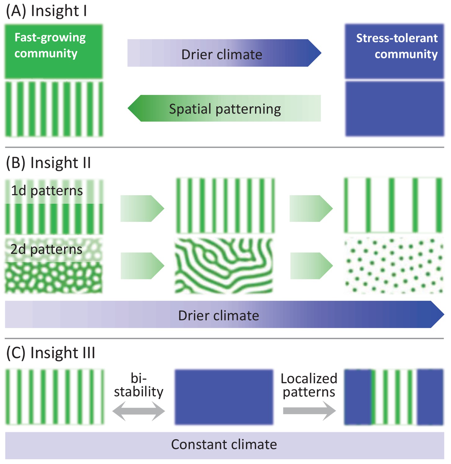
A schematic illustration of the three insights that the model study provides.
(A) Insight I: A drier climate shifts an original spatially uniform community of fast-growing plants, denoted by a green color, to a uniform community of stress-tolerant plants, denoted by blue color. Spatial patterning induced by the drier climate shifts the community back to fast growing plants. (B) Insight II: Once patterns have formed a yet drier climate has little effect on community structure – all patterned community states consist of fast-growing plants (green). This is because of further processes of spatial self-organization that increase the proportion of water-contributing bare-soil areas and compensate for the reduced precipitation. In one-dimensional (1d) patterns, these processes involve thinning of vegetation patches or transitions to longer wavelength patterns. In two-dimensional (2d) patterns, these processes involve morphological transitions from gap to stripe patterns and from stripe to spot patterns. (C) Insight III: Localized patterns in a bistability range of uniform and patterned community states significantly increase functional diversity, as they consist of both stress-tolerant (blue) and fast-growing (green) species. Such patterns can be formed by nonuniform biomass removal as an integral part of a provisioning ecosystem service.
Figure 2
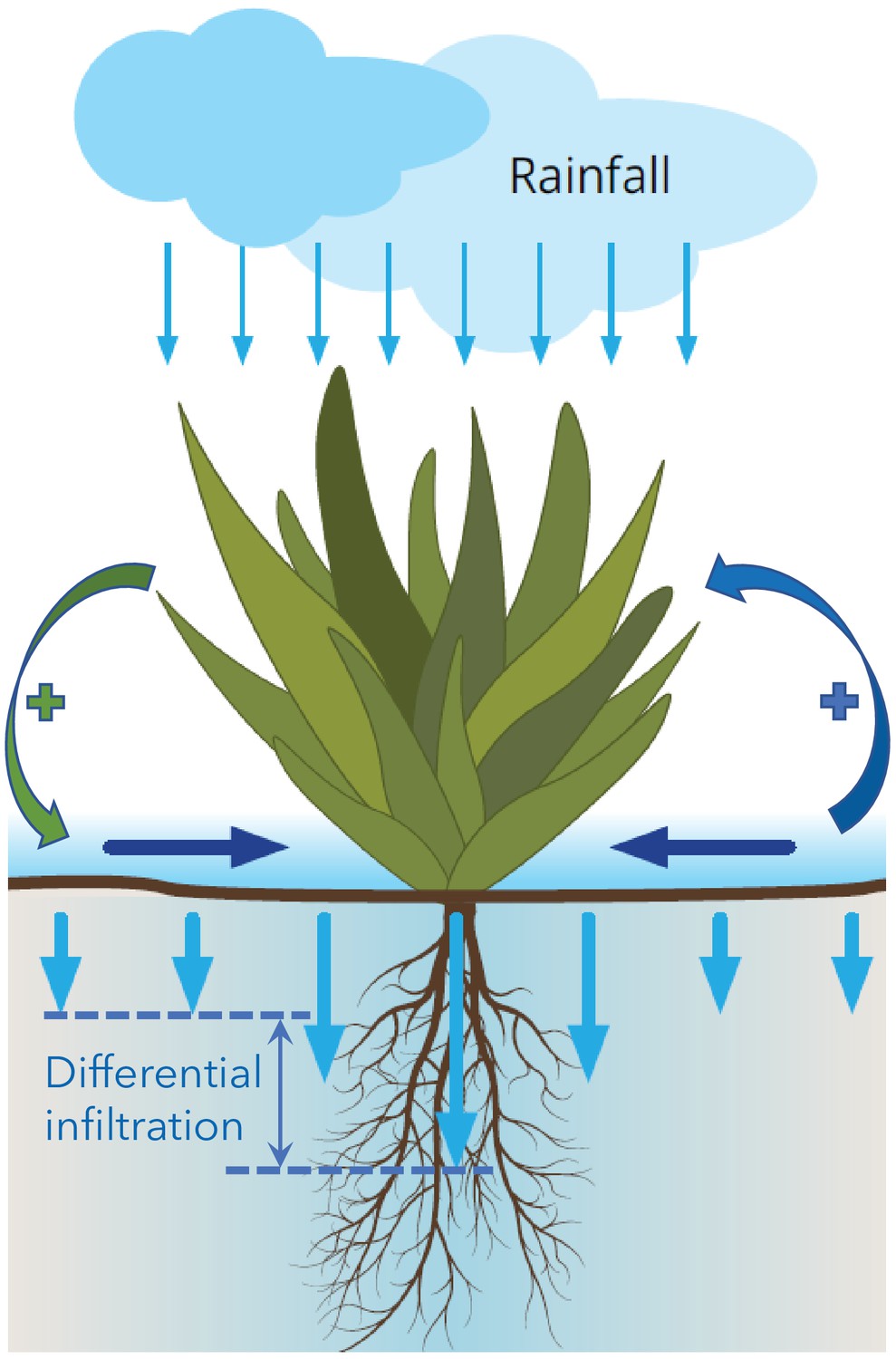
Illustration of overland water flow toward vegetation patches (horizontal arrows), induced by differential infiltration: low in bare soil (short vertical arrows) and high in vegetation patches (long arrows).
Vegetation growth enhances the infiltration contrast and thus the overland water flow (green round arrow), while that flow further accelerates vegetation growth (blue round arrow). The two processes form a positive feedback loop that destabilizes uniform vegetation to form vegetation patterns, and acts to stabilize these patterns once formed.
Figure 3
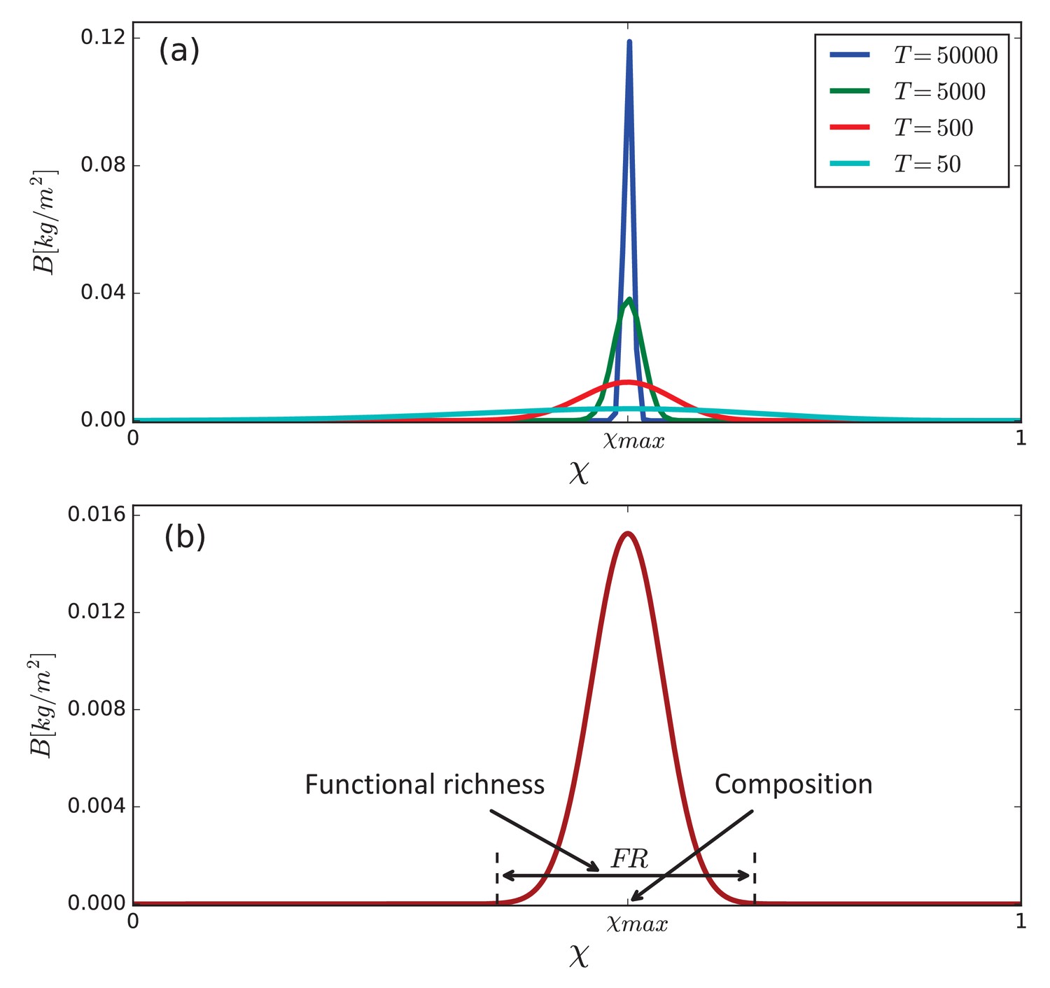
Emergence of a community as a stationary solution of the model Equations (1).
(a) Competitive exclusion of species in the course of time [y] when trait diffusion is not allowed (). (b) Asymptotic biomass distribution obtained with slow trait diffusion (). The distribution contains information about community-level properties such as community composition, quantified, among other metrics, by the position, , of the most abundant functional group, and functional richness, quantified, among other metrics, by the distribution width, , at small biomass values representing the biomass density of a seedling. Parameter values: mm/y and as stated in Table 1.
Figure 4
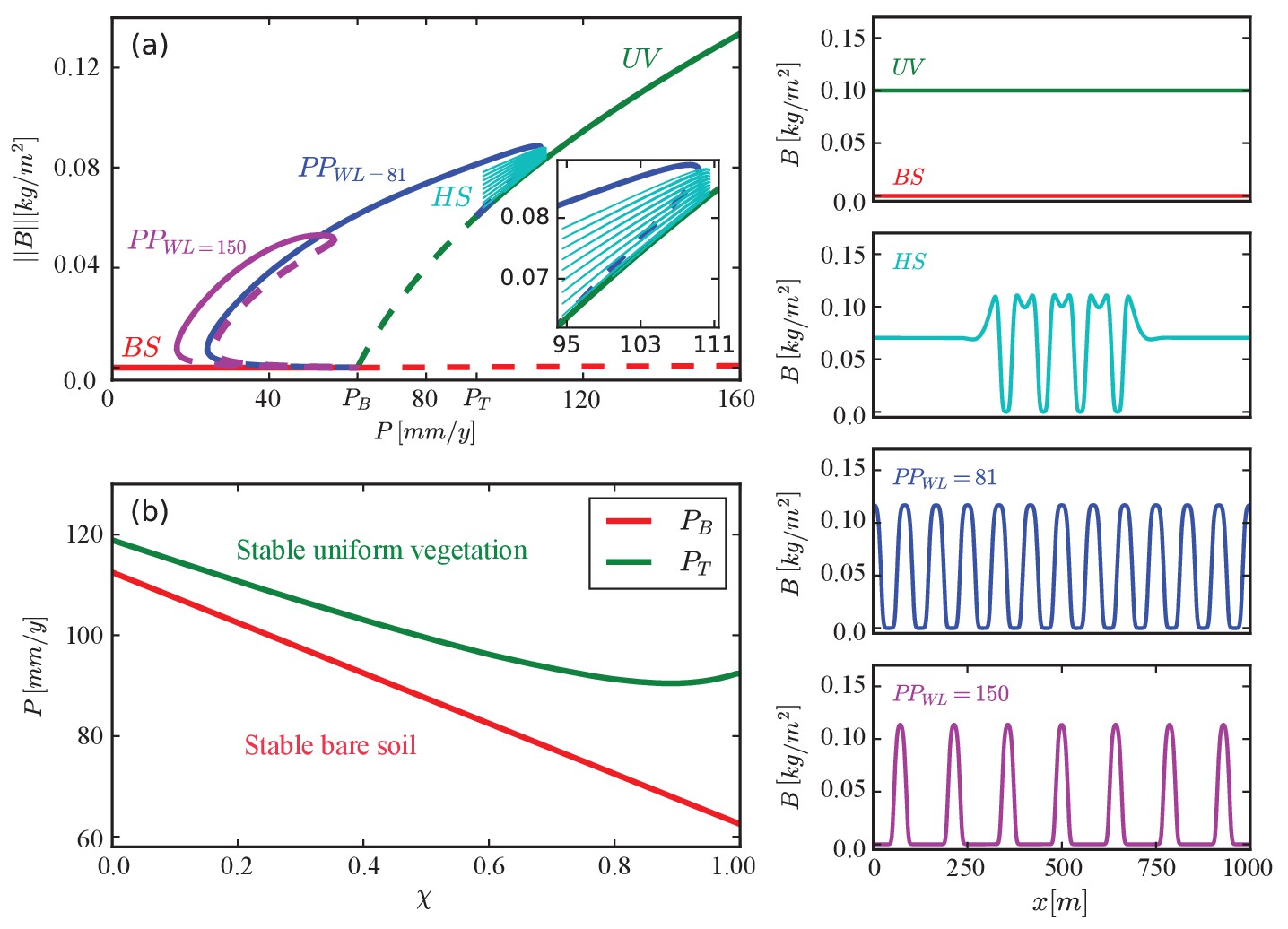
Existence and stability ranges of various solutions of a model for a single functional group.
(a) A bifurcation diagram showing the -norm of the biomass density vs. precipitation for . The colors and corresponding labels denote the different solution branches: uniform vegetation (), periodic patterns at different wavelengths (), hybrid states consisting of pattern domains in otherwise uniform vegetation (), and bare soil (). Solid (dashed) lines represent stable (unstable) solutions. Example of spatial profiles of these solutions are shown in the insets on the right. (b) Instability thresholds of uniform vegetation, , and of bare soil, , as functions of χ.
Figure 5
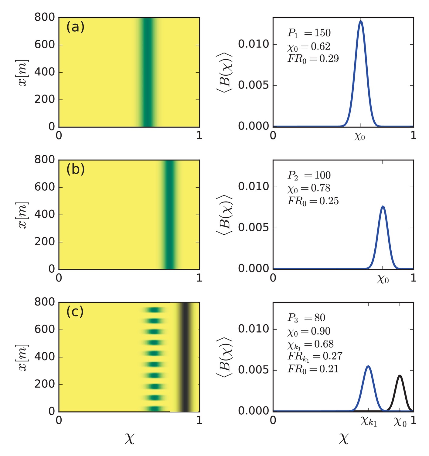
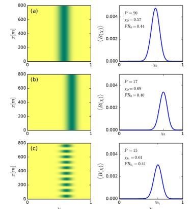
Community reassembly in response to precipitation downshifts.
Left panels show biomass distributions in the trait (χ) – space () plane for the specified precipitation rates . Right panels show biomass profiles along the χ axis averaged over space. (a,b) A precipitation downshift from mm/y to 100 mm/y, starting with a uniform community, results in a uniform community shifted to more tolerant species (higher χ), and of lower functional richness (). (c) Further decrease to mm/y results in a patterned community that is shifted back to species investing in growth (lower χ), and has higher functional richness. The biomass distributions in black refer to the unstable uniform community.
Figure 6
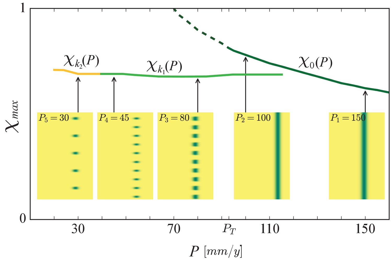
The buffering effect of spatial patterning on community structure.
Shown is a partial bifurcation diagram depicting different forms of community assembly along the precipitation axis, as computed by integrating the model equations in time. Stable, spatially uniform communities, (solid dark-green line), shift to stress-tolerant species (higher χ), as precipitation decreases. When the Turing threshold, , is traversed, spatial self-organization shifts the community back to fast-growing species (lower χ), and keep it almost unaffected as the fairly horizontal solution branches, (light green line), representing periodic patterns of wavenumber k1, and (yellow line), representing patterns of lower wavenumber k2, indicate. The insets show biomass distributions in the (χ, ) plane for representative precipitation values. The unstable solution branch describing uniform vegetation (dashed line) was calculated by time integration of the spatially decoupled model.
Figure 7
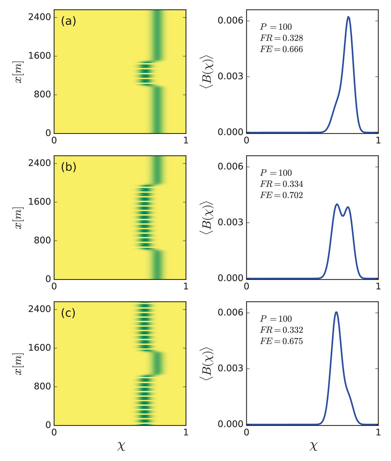
Increased functional diversity of hybrid states and evenness control.
Left panels show biomass distributions of different hybrid states in the trait (χ) – space () plane. Right panels show biomass profiles along the χ axis averaged over space. The functional richness, , of all hybrid states is almost equal and higher than that of purely uniform or purely patterned states (compare with panel b in Figure 5), but their functional evenness, , differs – high for patterned and uniform domains of comparable sizes (b) and low for small (a) and large (c) pattern-domain sizes. Calculated for a precipitation rate mm/y.
Author response image 1
Author response image 2
Tables
Table 1
Model paremeters, their descriptions, numerical values and units.
| Parameter | Description | Value | Unit |
|---|---|---|---|
| Growth rate at zero biomass | 0.032 | ||
| Water uptake rate | 20.0 | ||
| Infiltration contrast ( – high contrast) | 0.01 | - | |
| Maximal value of infiltration rate | 40.0 | ||
| Reference biomass at which for | 0.06 | ||
| L0 | Evaporation rate in bare soil | 4.0 | |
| Evaporation reduction due to shading | 10.0 | ||
| Capacity to capture light | variable | ||
| Minimal capacity to capture light | 0.1 | ||
| Maximal capacity to capture light | 0.6 | ||
| Mortality rate | variable | ||
| Minimal mortality rate | 0.5 | ||
| Maximal mortality rate | 0.9 | ||
| Relative contribution to infiltration rate | variable | - | |
| Minimal contribution to infiltration rate | 0.5 | - | |
| Maximal contribution to infiltration rate | 1.5 | - | |
| Precipitation rate | variable | ||
| χ | Tradeoff parameter | [0,1] | - |
| Number of functional groups | 128 | - | |
| Biomass dispersal rate | 1.0 | ||
| Soil-water diffusion coefficient | 102 | ||
| Overland-water diffusion coefficient | 104 | ||
| Trait diffusion rate | 10-6 |
Download links
A two-part list of links to download the article, or parts of the article, in various formats.
Downloads (link to download the article as PDF)
Open citations (links to open the citations from this article in various online reference manager services)
Cite this article (links to download the citations from this article in formats compatible with various reference manager tools)
Linking spatial self-organization to community assembly and biodiversity
eLife 10:e73819.
https://doi.org/10.7554/eLife.73819


