Toward the cellular-scale simulation of motor-driven cytoskeletal assemblies
- Center for Computational Biology, Flatiron Institute, United States
- Department of Physics, University of Colorado Boulder, United States
- Department of Molecular, Cellular, and Developmental Biology, University of Colorado Boulder, United States
- Courant Institute, New York University, United States
Figures
Figure 1 with 1 supplement
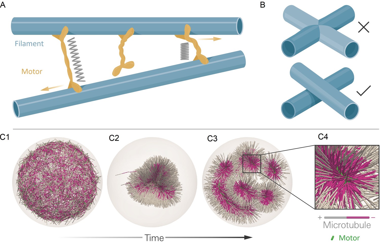
The computational model and demonstration of aLENS.
(A) aLENS simulates dynamics of rigid filaments crosslinked and driven by motors, thermal fluctuations, and steric interactions. Motors bind to, unbind from, and walk along filaments. (B) To achieve high efficiency, aLENS computes motor forces implicitly, and steric interactions through a novel geometric constraint method that avoids filament overlaps. (C1-C3) Example simulation of microtubules organized into asters by minus-end-directed motors. The 300 s Brownian simulation contains 3200 microtubules, each 1 µm long, inside a sphere of radius 3 µm. The initial position of each microtubule is random and the half of each filament on the minus-end is colored pink. Three end-pausing dynein motors are fixed at the minus-end of each microtubule and walk toward the minus-end of any microtubule they crosslink. After initial contraction into a single large aster, strong steric interactions in the aster center break up the system into several smaller asters and a bottle-brush structure. (C4) Motors are highly concentrated at the centers of asters.
Figure 1—video 1
Contraction and break-up of simulated microtubule asters.
The simulation details are described in Figure 1.
Figure 2
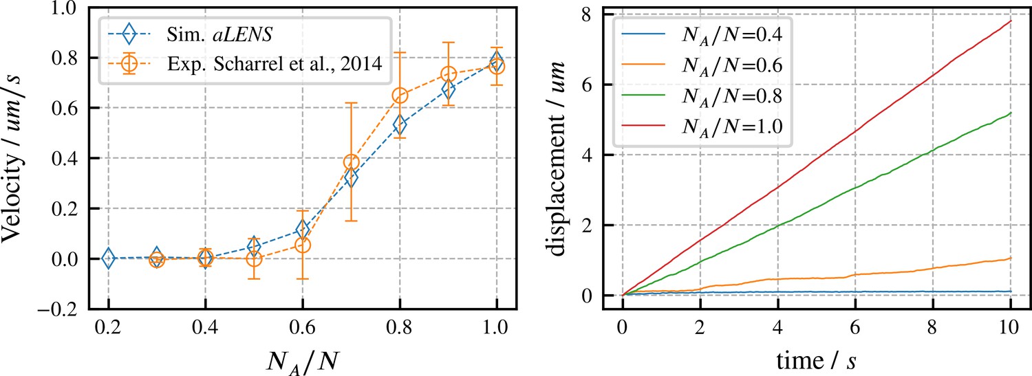
Directed transport velocity and displacement of microtubules driven by mixed active and inactive Kinesin-1 motors.
The total number of active and inactive motors is fixed at for all simulations. is the number of active motors. Left panel: comparison of microtubule velocities as a function of from aLENS simulations (blue diamonds) with from the reference experiment (orange circles) (Scharrel et al., 2014). Right panel: displacement vs. time of the transported microtubule obtained from simulation for several values of . The free walking velocity of active motors was set to to match the experimental sliding velocity at . There are no other fitting parameters. All motor parameters are estimates based on experiments on Kinesin-1 (Scharrel et al., 2014) or similar motor proteins (Cross and McAinsh, 2014).
Figure 3
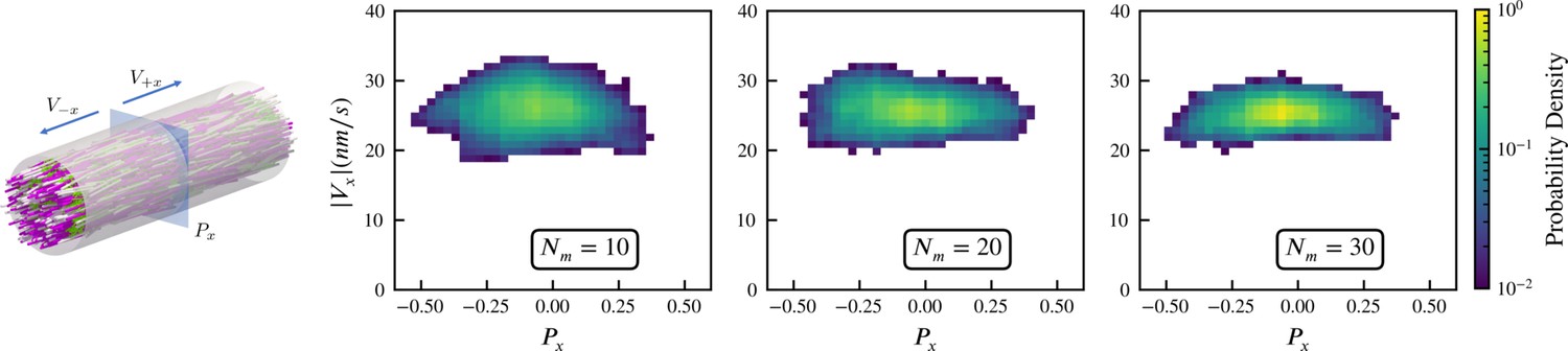
Sampled microtubule straining motion velocity vs local polarity in actively crosslinked microtubule network.
The left panel shows the simulation geometry and the sampling procedure. Microtubules are randomly initialized with orientations along the (pink) or (white) directions. XCTK2 motors are colored green. is the number of XCTK2 motors per microtubule. We sample the local average polarity and straining velocity by inserting planes orthogonal to the -axis into the collected data, matching the photobleaching technique used in experimental measurement (Fürthauer et al., 2019). For every sampling plane (e.g. the blue pane in the snapshot), we choose five sample points symmetrically on this plane and draw a square sampling window with edge length around each sample point. For each sampling window, we compute the average polarity along the -axis for all microtubules intersecting this sampling window at a given time. We then compute the velocities, averaged over (a duration chosen to match the experimental timescale), of microtubules intersecting each sampling window and moving along the and directions. and are computed from those two groups for each sampling window. The straining velocity is computed as . Therefore, for every sampling window at each sampling timestep we have a pair of data values . The right three panels show the joint probability distribution of computed from 900,000 sampling planes for each simulation, for , respectively.
Figure 4
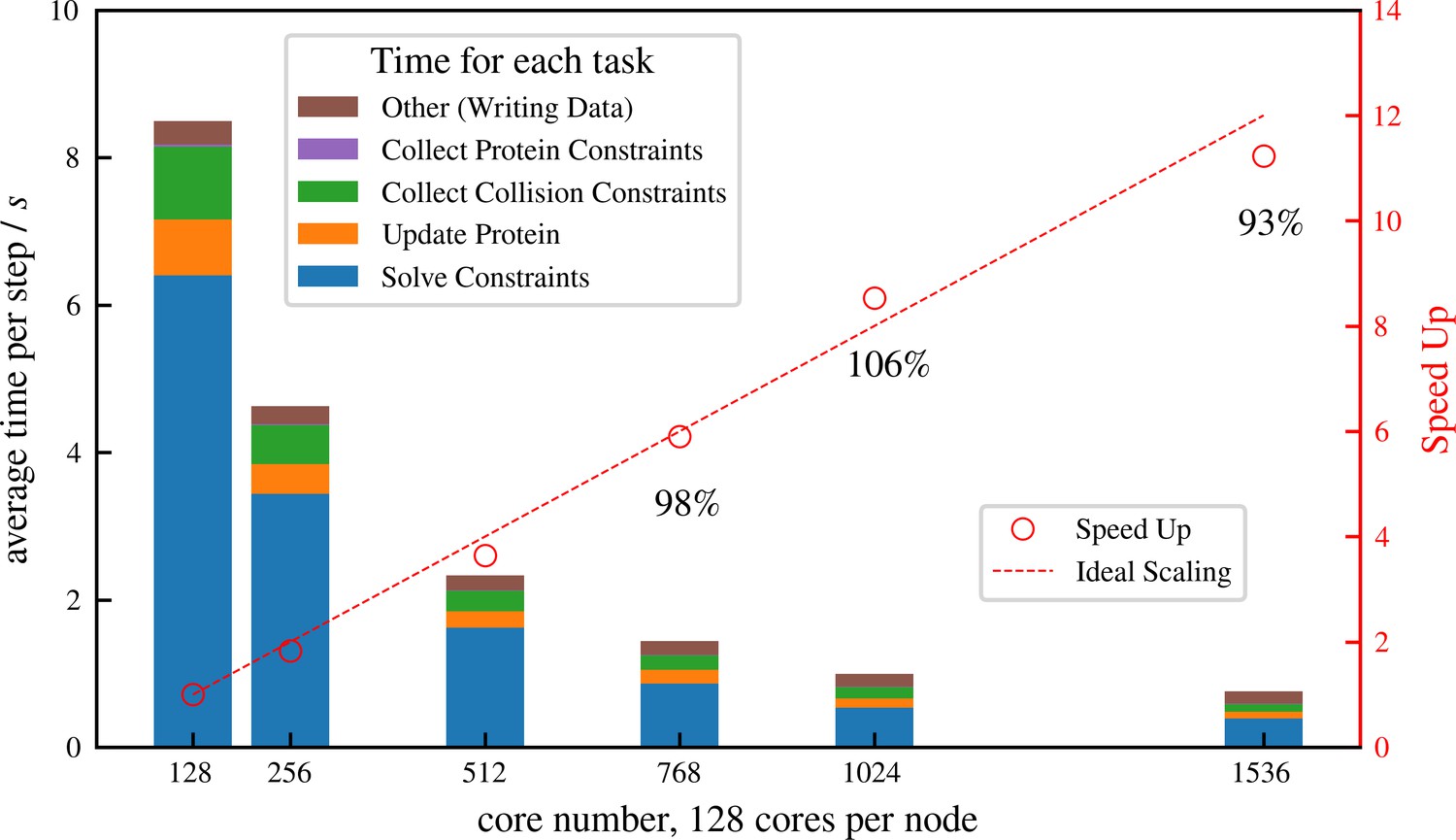
Strong scaling (fixed system size while increasing number of cores) efficiency of a system similar to but more than 10 times larger than that shown in Figure 6, comprising 1 million microtubules and 3 million motors.
There are in total approximately 8 million constraints per time step, which is changing from step to step because collision pairs are changing and crosslinkers are stochastically binding and unbinding. The simulation is run for 100 computing steps with 1 data-saving step and the average per-step wall-clock time is shown in the figure.
Figure 5 with 2 supplements
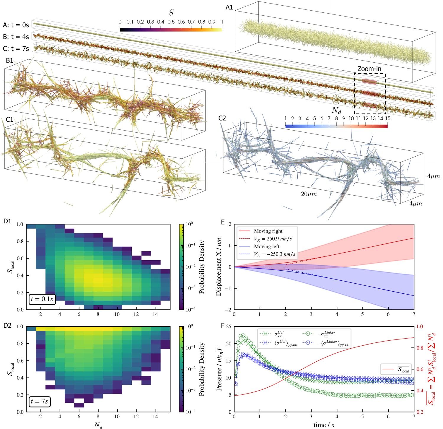
Results for the bundling-buckling simulation of 100,000 microtubules and 500,000 dynein motors in the periodic simulation box of .
Brownian motion of microtubules is turned off. Each dynein has one non-motile head permanently attached to a microtubule and the other motile head walks processively with maximum velocity . If bound, the motile head moves toward the microtubule minus-end, and detaches upon reaching it. Detailed parameters for this motor are tabulated in the Appendix 1. Every microtubule has 5 dynein motors permanently attached to randomly chosen, fixed locations along the length. The initial configuration of microtubules is randomly generated, with their orientations sampled from an isotropic distribution and centers uniformly distributed within a cylinder of length and diameter . The motile heads of all dynein motors are unbound initially. (A, B, C) The bundle at , , and . Microtubules are colored by their local nematic order parameter , with , being the unit orientation vector of each microtubule pointing from the minus to the plus end, and the Kronecker delta tensor. The average is taken over each microtubule plus all microtubules that are directly crosslinked to it by dynein motors. (A1, B1, and C1) Zoom-in views of the small region marked by red box in A, B, and C. (C2) The same region in C1 but colored by , the number of microtubules averaged over when computing . (D1 and D2) The joint probability distributions and for each microtubule for the entire systems at , when the dyneins crosslink microtubules but microtubules barely move from initial configuration, and at , when the bundle is nematic. (E) The average trajectories (solid lines) and their standard deviation (shaded area) of left-moving and right-moving microtubules. Dashed lines show linear fits to the average trajectory after , with results . (F) The normal stresses and the weighted average over time. Due to the symmetry in the directions, only their average is shown . Collision stress is positive (extensile) and crosslinker stress is negative (contractile). The weighted average .
Figure 5—video 1
Contraction and buckling of a long microtubule-motor bundle.
The bottom panel is a zoom-in view to the area in a gray box in the top panel. The simulation details are described in Section Bundle formation and buckling in a filament band.
Figure 5—video 2
Motor motion and stretching during the contraction and buckling of a long microtubule-motor bundle.
This is a zoom-in view to the area in a gray box in the bottom panel in Figure 5—video 1. The simulation details are described in Section Bundle formation and buckling in a filament band.
Figure 6
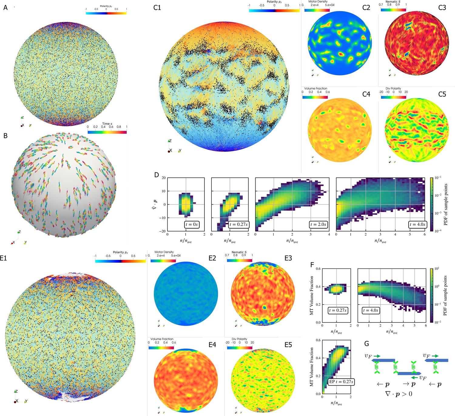
Results for the polarity sorting simulation in a spherical shell.
Initially, 100,000 0.25 µm-long filaments modeling microtubules and 200,000 motors modeling crosslinking kinesin-like proteins are placed between two concentric spherical shells with radii and , to maintain the volume fraction of filaments between these two shells at 40%. Initially, all filaments are evenly distributed on the spherical shell, with their orientation randomly chosen to be either at each point, where is the polar basis norm vector of spherical coordinate system. The pure filament system is relaxed for to resolve the overlaps in the initial configuration. Afterwards at , motors are added to the system homogeneously distributed between the two shells. Sample points are evenly placed to measure the statistics by averaging the volume within from each sample point. (A) The configuration at . Filaments are colored by their polarity, while motors are colored as black dots. Only randomly selected 10% of all motors (same after) are shown in the image to illustrate the distribution. (B) Randomly selected trajectories of filaments from to . Trajectories are colored by time. It is clear that filaments move along the meridians. (C1-C5) Configuration and statistics at . (C1) The filaments and motors. Motors clearly concentrate in some areas. (C2) The motor number density, that is, number of motors per . (C3) The nematic director field (shown as black bars) and the nematic order parameter . (C4) The filament volume fraction. (C5) The divergence of polarity field non-dimensionalized by filament length, that is, change of mean polarity per filament length. (D) The development of the correlation between motor number density and the polarity divergence field, at different times of the simulation. Clearly high are correlated with positive polarity divergence. (E1-E5) Configuration and statistics at for a comparative simulation where motors have end-pausing, arranges in the same style as C1-C5. This case shows significant contraction instead of polarity sorting as filaments are pulled away from the north and south poles and the overall volume fraction significantly increases to approximately 60%. The structure becomes densely packed and does not significantly evolve further. (F) The correlation between motor number density and the local filament volume fraction. For the polarity sorting case at the motor number density correlates with low filament volume fraction. This is not seen in the end pausing (EP) case. (G) A schematic for the correlations shown in D and F.
Figure 7 with 2 supplements
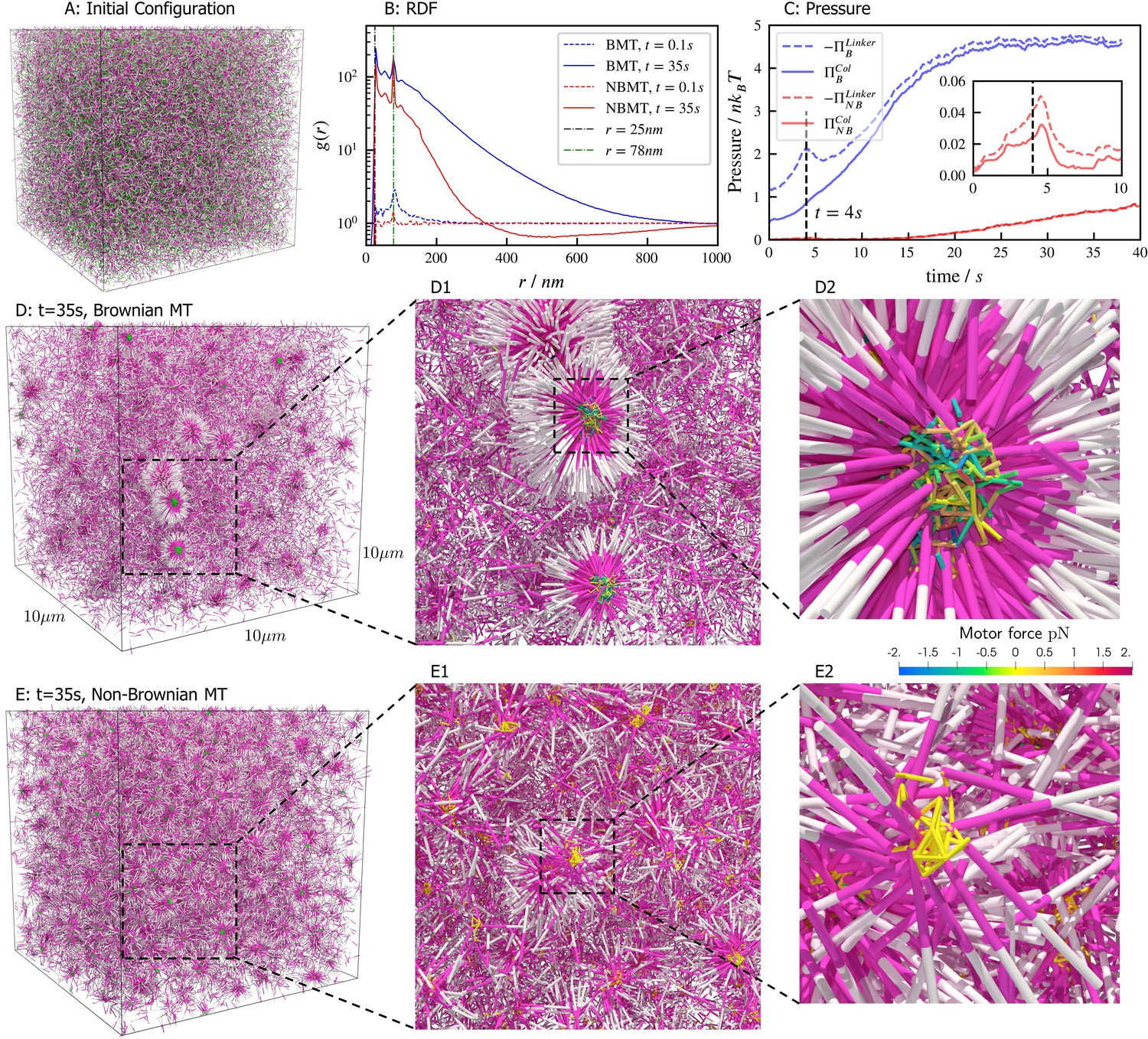
Results for the aster formation simulations with Brownian motion of simulated microtubules turned on (BMT) and off (NBMT).
Initially, 40,000 -long filaments modeling microtubules and 80,000 motors modeling crosslinking kinesin-like proteins are placed in a periodic cubic box of with uniform distribution. Filament orientations are isotropic and motors are all in the unbound state. Motors are assumed to have two minus-end-directed walking heads with symmetric properties. They are assumed to pause when they reach the minus end of filaments until detaching. Detailed parameters are tabulated in Appendix B. (A, D, and E) Simulation snapshots. Each filament is shown as a cylinder colored in half pink (minus end) and half white (plus end). (A) The initial configuration for both NMT and BNMT cases. Each motor is colored as a green dot. (D and E) The snapshot for both cases at . D1-2 and E1-2 Expanded views of a aster core for D and E. Only doubly bound motors are shown in D and E (in green color), and in D1-2 and E1-2 (colored by the spring force). Negative values mean the crosslink forces are contractile (attractive). (B) The radial distribution function (RDF) for the minus ends of all filaments at (dashed lines) and (solid lines). The first peak of at corresponds to close contacts between filaments. The second peak of at corresponds to the minus ends of filaments crosslinked by motors whose rest length is . Blue and red lines are results for the BMT and NBMT cases, respectively. (C) The collision (solid) and crosslinker (dashed) pressure for BMT (blue) and NBMT (red) cases. Pressure is defined as the trace of the stress tensor: . The collision pressure is positive (extensile), and the motor pressure is negative (contractile). The inset plot shows the pressure for the NBMT case in the initial stage of the simulation. The black dashed lines mark the time .
Figure 7—video 1
Aster formation in bulk of Brownian microtubules.
This is a zoom-in view to the BMT case shown in Figure 7.
Figure 7—video 2
Aster formation in bulk of Non-Brownian microtubules.
This is a zoom-in view to the NBMT case shown in Figure 7.
Figure 8 with 2 supplements
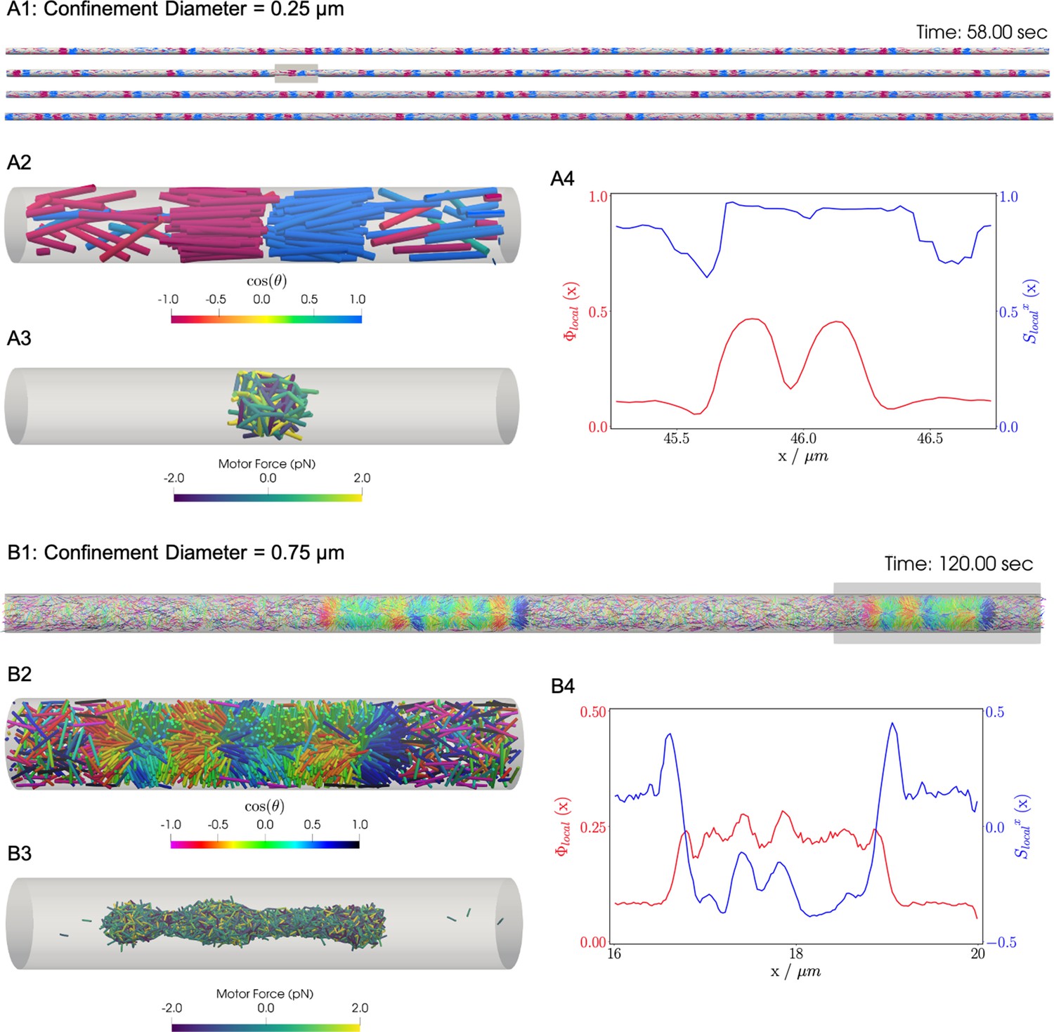
Results for the confined filament-motor protein assembly simulations with filaments modeling microtubules and motors modeling crosslinking kinesin-like proteins at a cylinder diameter of and .
Initially, long filaments are uniformly distributed and aligned along the -axis, with equal numbers oriented in the and directions. Crosslinking motor proteins are initially unbound and distributed uniformly as well. A and B: Snapshots of the simulation with and at and . A1 and B1: All 9,216 simulated filaments. In A1, the the cylinder is too long to be displayed contiguously, therefore a stacked representation is shown. The filaments are colored by the value of where θ is the angle between the filament direction vector (oriented from the minus-end to the plus-end) and the positive -axis (pointing to the right). A2 and B2: Zoomed-in view of the filaments in the boxed regions in A1 and B1. A3 and B3: Doubly-bound motors in the boxed regions, colored by their binding force. Negative values represent contractile force while positive values indicate extensile force. A4 and B4: The local packing fraction (red line) and the local nematic order parameter (blue line), where a filament contributes to the local order at . Filament contributions are weighted by and summed over all filaments at . Line plots represent an average over for the snapshots in A2 and B2. Detailed parameters and calculations for the crosslinking motor proteins are presented in Appendix G.
Figure 8—video 1
Filament-motor assembly for the case.
The bottom panel is a zoom-in view to the area in a gray box in the top panel. The simulation details are described in Section Confined filament-motor protein assemblies.
Figure 8—video 2
Filament-motor assembly for the case.
The bottom panel is a zoom-in view to the area in a gray box in the top panel. The simulation details are described in Section Confined filament-motor protein assemblies.
Appendix 2—figure 1
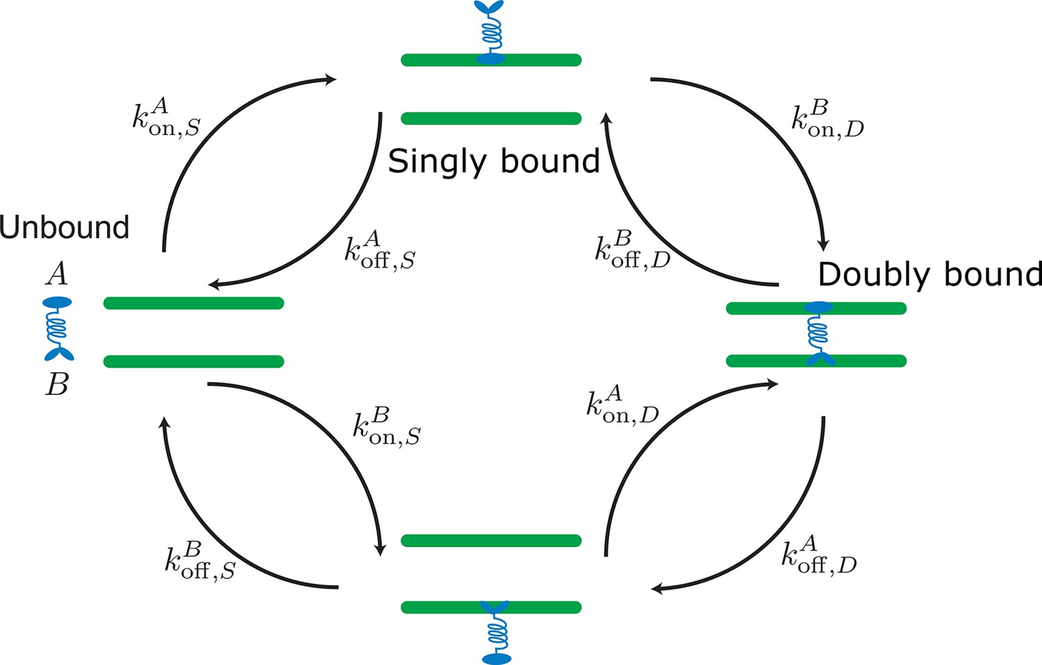
Labels and definition of kinetic rates for crosslinking proteins binding to filaments (green) implemented in the kinetic Monte Carlo algorithm.
Crosslinking proteins (blue) exist in three different states: neither head attached to a filament (unbound), bound with one head attached to a filament (singly bound), and crosslinking two filaments (doubly bound). Motors and crosslinkers may have different rates for separate binding heads (A,B).
Appendix 2—figure 2

Comparison of initially unbound passive crosslinkers binding to a filament with binding radii set to a crosslinker’s radius of gyration versus a binding radius .
(A, D) Number of singly bound crosslinkers over time as the unbound diffusion constant (A) and time step (D) vary while binding radius remains unchanged . Red lines mark the steady-state number of singly bound crosslinkers for a homogeneous reservoir calculated from equations (26)-(30). (B, E) Same as A and D but binding radius scales as the root mean square of diffused distance in a time step . (C, F) Comparison of the steady-state number of singly bound crosslinkers as a function of (C) and (F) for both definitions of . Simulation parameters: periodic box length , filament length , linear binding site density , crosslinker number , crosslinker length , association constant , unbinding rate . Unless otherwise stated unbound diffusion constant and timestep
Appendix 3—figure 1
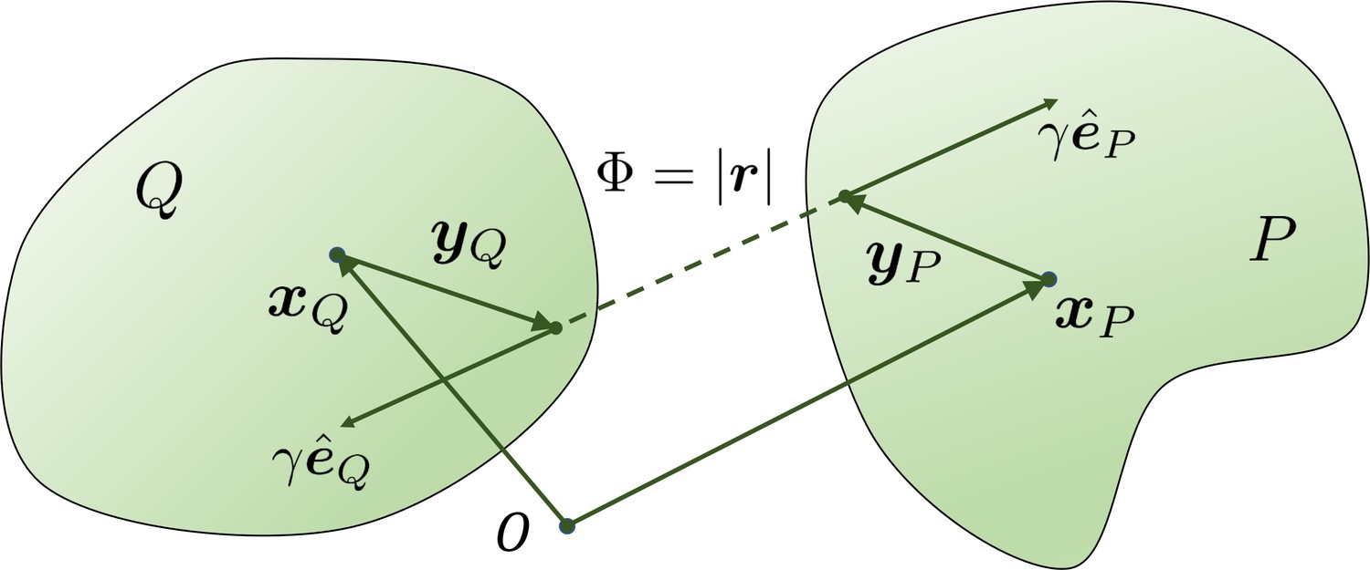
The geometry for a pair of rigid particles.
The distance between two marked points , where .
Appendix 4—figure 1
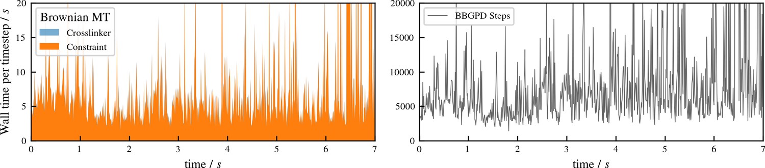
Performance of aLENS for the buckling simulation shown in Figure 5 of main text.
The left panel shows the wall clock time that every timestep takes. The right panel shows the number of BBPGD steps to solve the constraint optimization problem at every timestep.
Appendix 4—figure 2
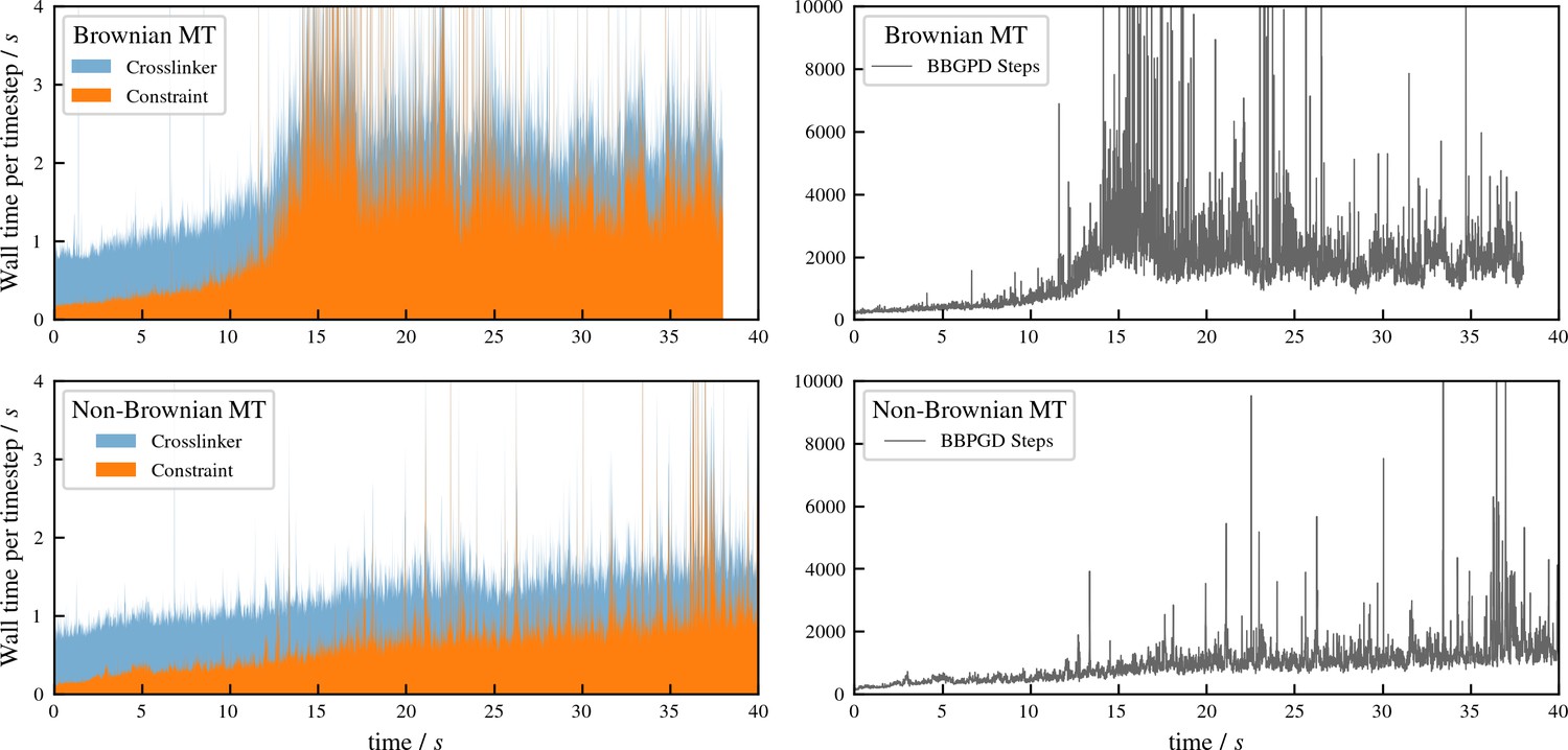
Performance of aLENS for aster formation simulations shown in Figure 7 of main text.
The left panels show the wall clock time that every timestep takes to simulate the Brownian and Non-Brownian cases. The right panels show the number of BBPGD steps to solve the constraint optimization problem at every timestep for those two cases.
Appendix 5—figure 1
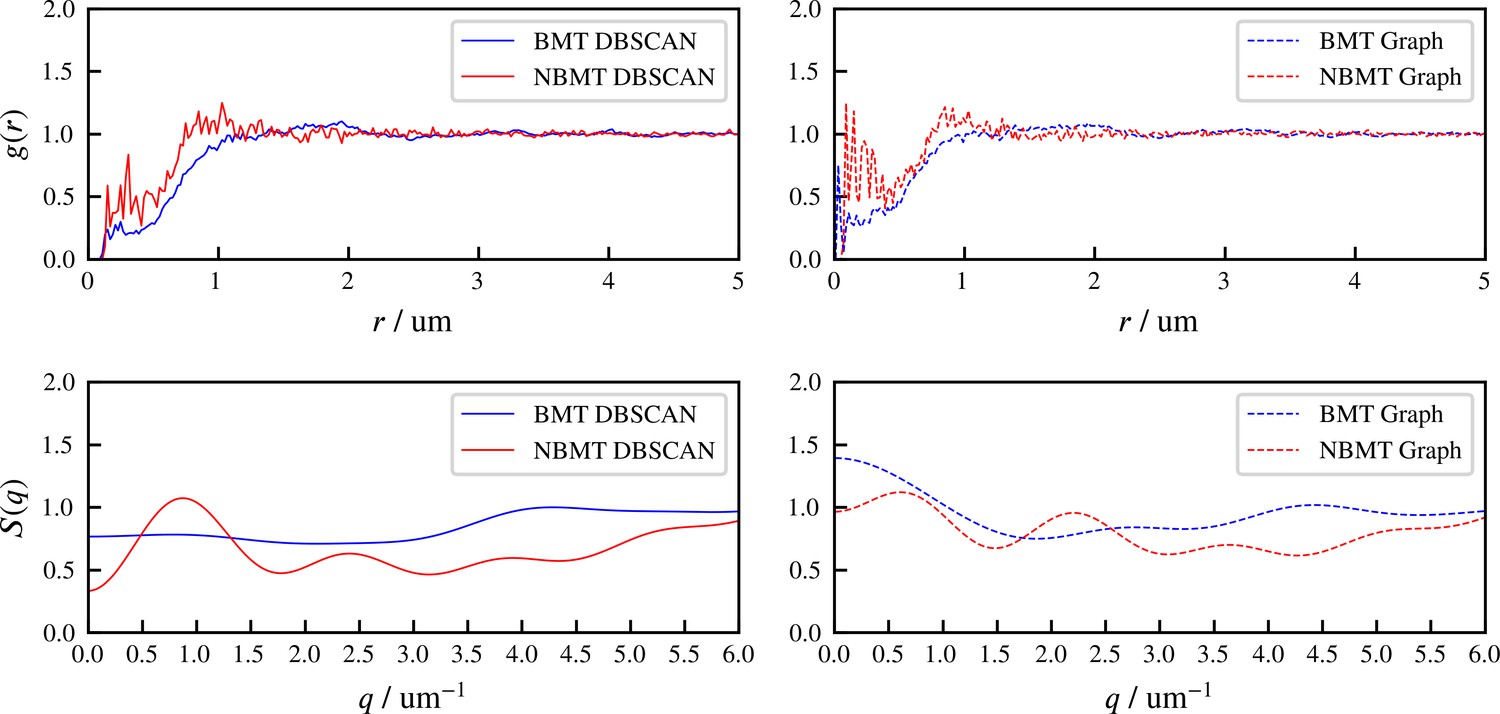
The radial distribution function and structure factor of identified aster centers at steady state, for BMT and NBMT cases.
‘DBSCAN’ and ‘Graph’ refer to two different methods of identifying aster centers, based on spatial locations of all microtubule minus ends, and the crosslinking connectivity, respectively. 500 snapshots at simulation steady state are used to compute and , for each case.
Appendix 6—figure 1
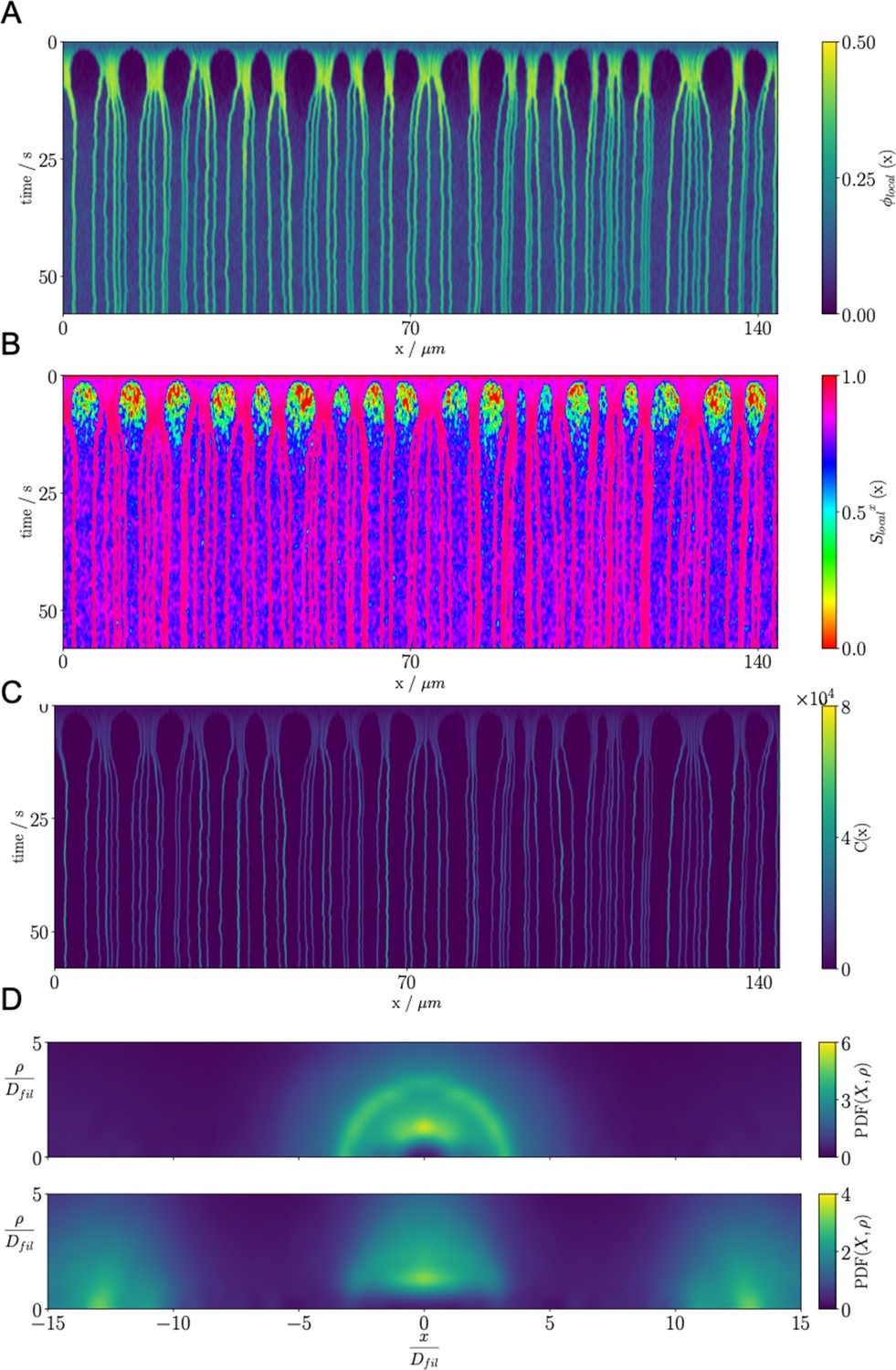
Results for the confined microtubule-motor protein assembly simulations with .
(A) A kymograph of the local microtubule packing fraction . Initially, crosslinking motor proteins drive contraction of the system into condensed regions that break into PSBs over time. (B) A kymograph of the local nematic order parameter . (C) A kymograph of the density of the crosslinking motor proteins, . Condensation of microtubules coincides with condensation of the crosslinking motor proteins. (D) Pair distribution function for microtubule plus-ends (top) and microtubule centers (bottom).
Appendix 6—figure 2

Results for the confined microtubule-motor protein assembly simulations with .
(A) A kymograph of the local microtubule packing fraction . Crosslinking motor proteins drive contraction of the system. Self organization of these regions leads to emergence of the BB-like state. (B) A kymograph of the local nematic order parameter . The negative order parameter suggests that there is alignment of microtubules in the radial direction ( plane). (C) A kymograph of the density of the crosslinking motor proteins, . (D) Pair distribution function for microtubule plus-ends (top) and microtubule centers (bottom).
Appendix 6—figure 3
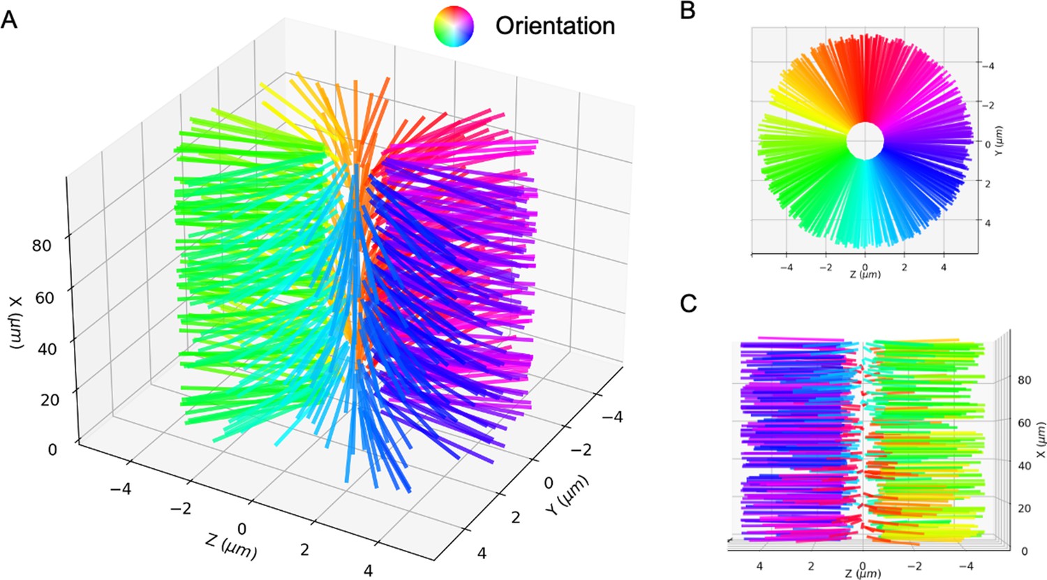
The perfect bottle-brush state.
Microtubules are aligned in the planes such that there is a line defect along the axis. (A) 3D view. (B) Side view. (C) Top view. Microtubule orientation is shown by the color wheel.
Appendix 7—figure 1
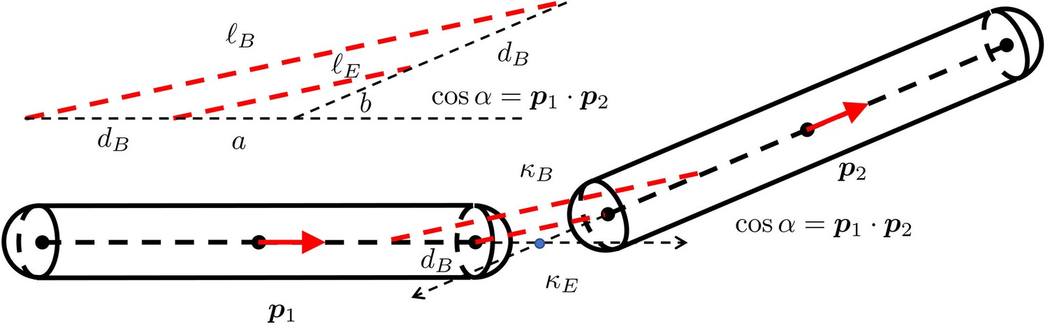
The geometry of two short rigid straight fibers connected at a bending joint.
The separation is exaggerated to clearly show the geometry. and are the orientation norm vectors of the two segments. and are the stiffness of the spring for extension and the spring for bending. is the displacement distance from the joint rotation center. In the more detailed view of the deformed geometry of the two springs, are the lengths of the two edges of the triangle. . .
Appendix 7—figure 2
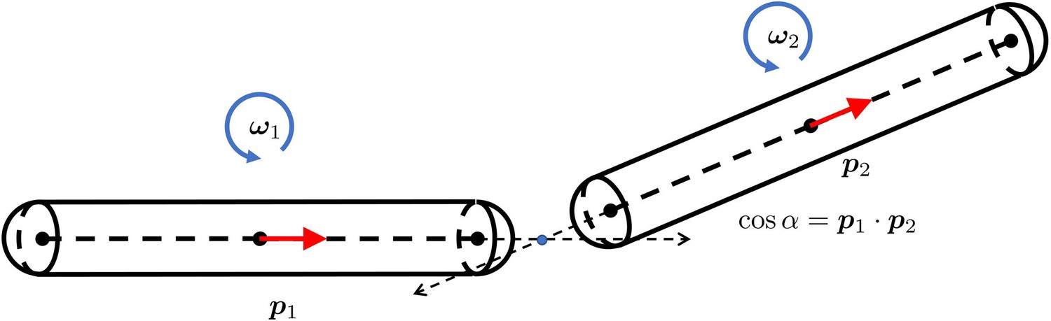
The geometry of two short rigid straight fibers connected at a bending joint.
The separation is exaggerated to clearly show the geometry. and are the orientation norm vectors of the two segments. and are the rotational angular velocities. is the bending energy of this joint. α is the angle from to . E is the bending rigidity modulus.
Author response image 1
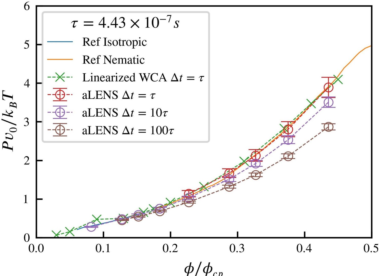
Comparison of the equation of state for 1µm microtubules at room temperature across the isotropicnematic transition range of volume fractions.
ϕcp = 0.9036 is the close packing volume fraction. The reference data is adapted from [7], generally accepted as the ground truth for rigid Brownian liquid crystal equation of state. Simulations using linearized WCA potential uses the code by [8], which has a constant repulsive force when the distance between rods is smaller than 0.812DMT, where DMT is the microtubule diameter.
Tables
Table 1
The transition rates between all possible states of a crosslinker .
means either head or is bound but the other is unbound. All binding rates account for the linear binding density is the length of filament with center-of-mass position and orientation inside the capture sphere with cutoff radius relative to position of motor/crosslinker . The sum is over all possible candidate filaments . The unbound-singly bound transition is determined by the association constant and the force-independent off rate . Similarly, the singly bound-doubly bound transition is determined by the association constant and force-independent off rate is the Boltzmann factor. in the in the transition rates refers to the tether energy of a motor . is the free length of a motor, while is the length for computing the force when attached to filaments and at locations si and sj: ). The dimensionless factor λ determines the energy dependence in the unbinding rate. Both binding and unbinding rates must depend on λ and such that the equilibrium constant recovers the Boltzmann factor For force-dependent binding models, the can be simply replaced by the tether force . This is not used for results shown in this work, but implemented in the code.
| Process | Rate | Value |
|---|---|---|
Appendix 1—table 1
The parameters of the two springs controlling extension and bending, respectively.
| Parameter | Explanation | Unit |
|---|---|---|
| End-pausing | True or False | ND |
| One head fixed | True or False | ND |
| λ | energy factor | ND |
| parallel to anti-parallel factor | ND | |
| free length | ||
| rc | capture radius | |
| κ | Hookean spring constant | |
| stall force | ||
| unbound diffusivity | ||
| binding site density | ||
| vm | max walking velocity | |
| association constant () | ||
| off-rate constant () | ||
| effective association constant () | ND | |
| force-independent off-rate constant () | ||
| singly bound head diffusivity | ||
| doubly bound head diffusivity | ||
| singly bound walking velocity | ||
| xc | force-dependent unbinding length |
Appendix 1—table 2
Properties of crosslinkers used in the main text.
ND means dimensionless. Parameters given as an array means the two values are used for each each of a crosslinker, respectively. Kinesin-5 parameters are adapted from Blackwell et al., 2017. Dynein parameters are adapted from Foster et al., 2017. Kinesin-1 parameters are adapted from Scharrel et al., 2014.
| Parameter | Kinesin-5 | Dynein | Kinesin-1 | Inactivated Kinesin-1 |
|---|---|---|---|---|
| End-pausing | True | False | False | False |
| One head fixed | False | True | True | True |
| λ | 0.258 | 0.5 | 0.5 | 0.5 |
| 1 | 1 | 1 | 1 | |
| 0.053 | 0.040 | 0.05 | 0.05 | |
| rc | 0.039 | 0.033 | 0.038 | 0.038 |
| κ | 300.0 | 100.0 | 100.0 | 100.0 |
| 5.0 | 1.0 | 7.0 | 7.0 | |
| 1.0 | 1.0 | 1.0 | 1.0 | |
| 0 | 0 | |||
| 0 | 0 | |||
| 1,625 | 400 | 400 | 400 | |
| vm | ||||
Appendix 2—table 1
The transition rates between all possible states of a crosslinker .
means either head or is bound but the other is unbound. All binding rates account for the linear binding density is the length of filament with center-of-mass position and orientation inside the capture sphere with cutoff radius relative to position of motor/crosslinker . The sum is over all possible candidate filaments . The unbound-singly bound transition is determined by the association constant and the force-independent off rate . Similarly, the singly bound-doubly bound transition is determined by the association constant and force-independent off rate with an additional factor , the effective volume explored by the unattached head while the motor/crosslinker is singly bound. Energy dependence in the transition rates is imposed by the Boltzmann factor that is a function of , the tether length of the motor/crosslinker attached to filaments and at locations si and sj), the characteristic length of the tether not under load , and the filament diameter . The dimensionless factor λ determines the energy dependence in the unbinding rate while the xc is the characteristic length that determines the force dependence. The latter is not used in the simulations of the main text but is implemented in the code base.
| Process | Rate | Value |
|---|---|---|
Appendix 7—table 1
The parameters of the two springs controlling extension and bending, respectively.
The relation between and determine the equilibrium configuration of the two connected filaments. When , the straight configuration is the preferred configuration.
| Role | spring stiffness constant | free length |
|---|---|---|
| Bending | ||
| Extension |
Download links
A two-part list of links to download the article, or parts of the article, in various formats.
Downloads (link to download the article as PDF)
Open citations (links to open the citations from this article in various online reference manager services)
Cite this article (links to download the citations from this article in formats compatible with various reference manager tools)
Toward the cellular-scale simulation of motor-driven cytoskeletal assemblies
eLife 11:e74160.
https://doi.org/10.7554/eLife.74160


