A neural network model of when to retrieve and encode episodic memories
- Department of Psychology, Princeton University, United States
- Princeton Neuroscience Institute, Princeton University, United States
Figures
Figure 1
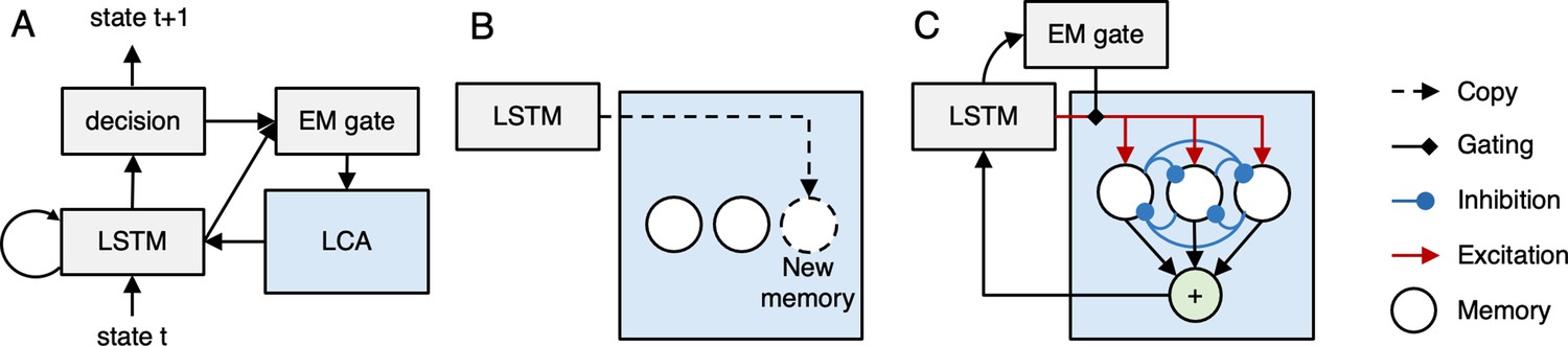
Neocortical-hippocampal Model.
(A) At a given moment, the neocortical part of the model (shown in gray) observes the current state and predicts the upcoming state. It incorporates a Long Short Term Memory (LSTM; Hochreiter and Schmidhuber, 1997) network, which integrates information over time; the LSTM feeds into a non-linear decision layer. The LSTM and decision layers also project to an episodic memory (EM) gating layer that determines when episodic memories are retrieved (see part C of figure). The entire neocortical network is trained by an advantage-actor-critic (A2C) objective (Mnih et al., 2016) to optimize next-state prediction. (B) Episodic memory encoding involves copying the current hidden state and appending it to the list of memories stored in the episodic memory system (shown in blue), which is meant to correspond to hippocampus. (C) Episodic memory retrieval is implemented using a leaky competing accumulator model (LCA; Usher and McClelland, 2001) – each memory receives excitation proportional to its similarity to the current hidden state, and different memories compete with each other via lateral inhibition. The EM gate (whose value is set by the EM gate layer of the neocortical network) scales the level of excitation coming into the network. After a fixed number of time steps, an activation-weighted sum of all memories is added back to the cell state of the LSTM.
Figure 2
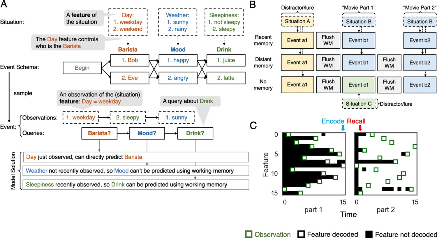
A situation-dependent event processing task.
(A) An event is a sequence of states, sampled from an event schema and conditioned on a situation. An event schema is a graph where each node is a state. A situation is a collection of features (e.g., Day, Weather, Sleepiness) set to particular values (e.g., Day = weekday). The features of the current situation deterministically control how the event unfolds (e.g., the value of the Day feature controls which Barista state is observed). At each time point, the network observes the value of a randomly selected feature of the current situation, and responds to a query about what will happen next. Note that the order of queries is fixed but the order in which situation features are observed is random. If a situation feature (Sleepiness) is observed before the state it controls (Drink), the model can answer the query about that state by holding the relevant feature in working memory. However, if the relevant situation feature (Weather) is observed after the state it controls (Mood), the model can not rely on working memory on its own to answer the query. (B) We created three task conditions to simulate the design used by Chen et al., 2016: recent memory (RM), distant memory (DM), and no memory (NM); see text for details. (C) Decoded contents of the model’s working memory for an example trial from the DM condition. Green boxes indicate time points where the value of a particular situation feature was observed. The color of a square indicates whether the correct (i.e., observed) value of that feature can be decoded from the model’s working memory state (white = feature accurately decoded; black = feature not decoded). See text for additional explanation.
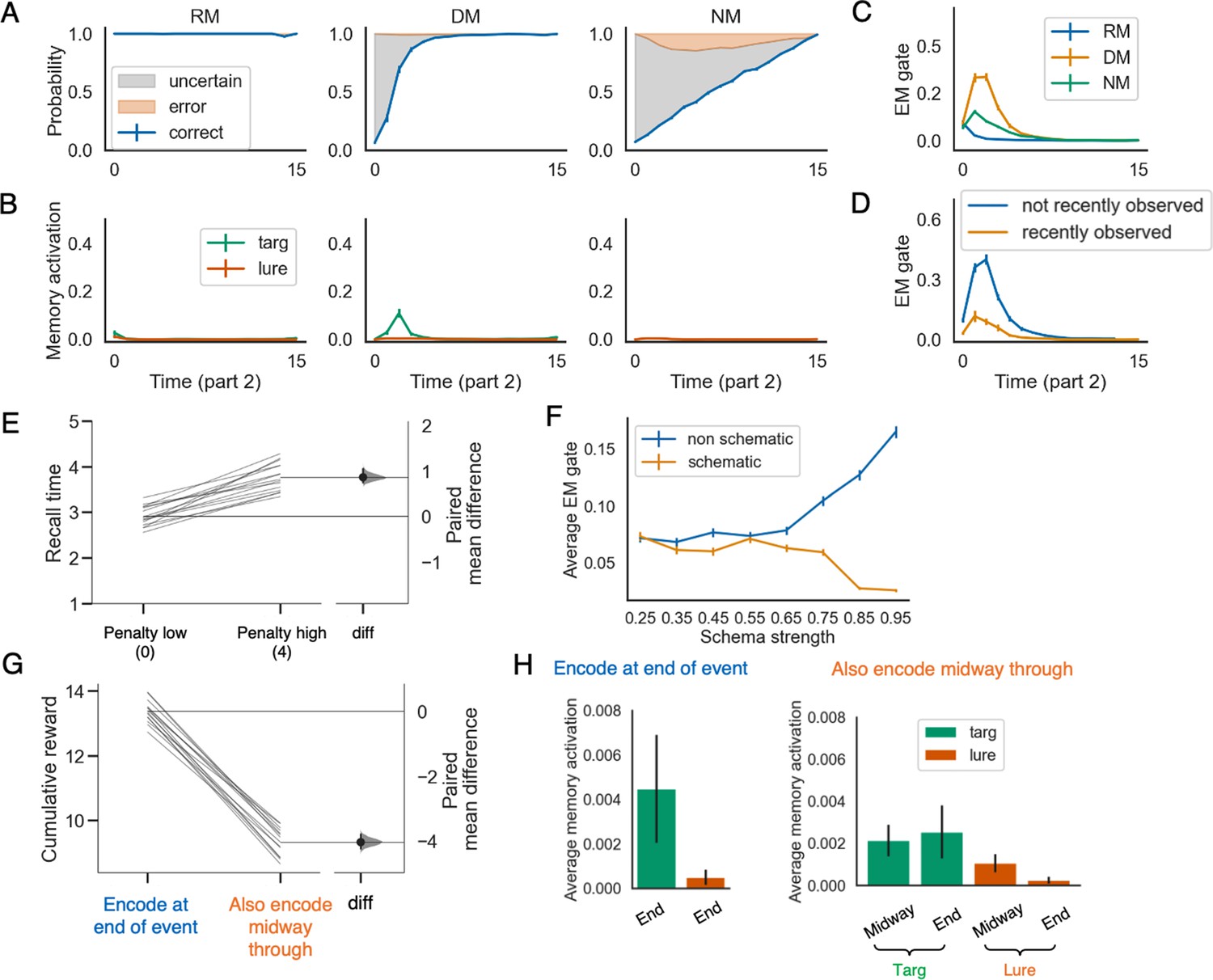
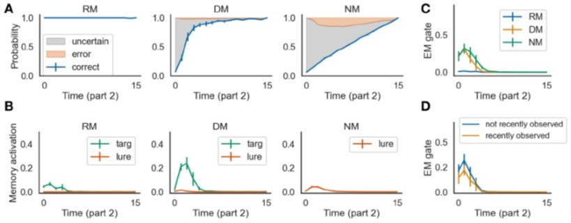
Figure 3
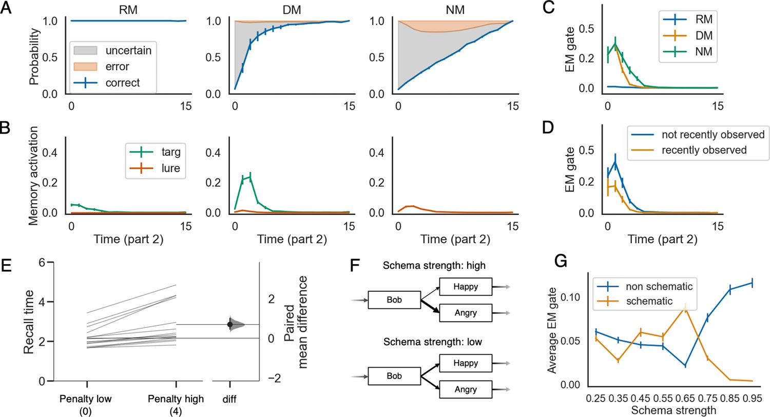
The learned episodic retrieval policy is selective.
Panels A, B and C show the model’s behavioral performance, memory activation, and episodic memory gate (EM gate) value during part 2, across the recent memory (RM), distant memory (DM), and no memory (NM) conditions, when the penalty for incorrect prediction is set to two at test. These results show that recall is much stronger in the DM condition (where episodic retrieval is needed to fill in gaps and resolve uncertainty) compared to the RM condition. (D) shows that, in the DM condition, the EM gate value is lower if the model has recently (i.e., in the current event) observed the feature that controls the upcoming state transition. (E) shows how the average recall time is delayed when the penalty for making incorrect predictions is higher. (F) illustrates the definition of the schema strength for a given time point. (G) shows how the average EM gate value changes as a function of schema strength (penalty level = 2). The errorbars indicate 1SE across 15 models.
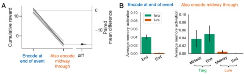
Figure 4
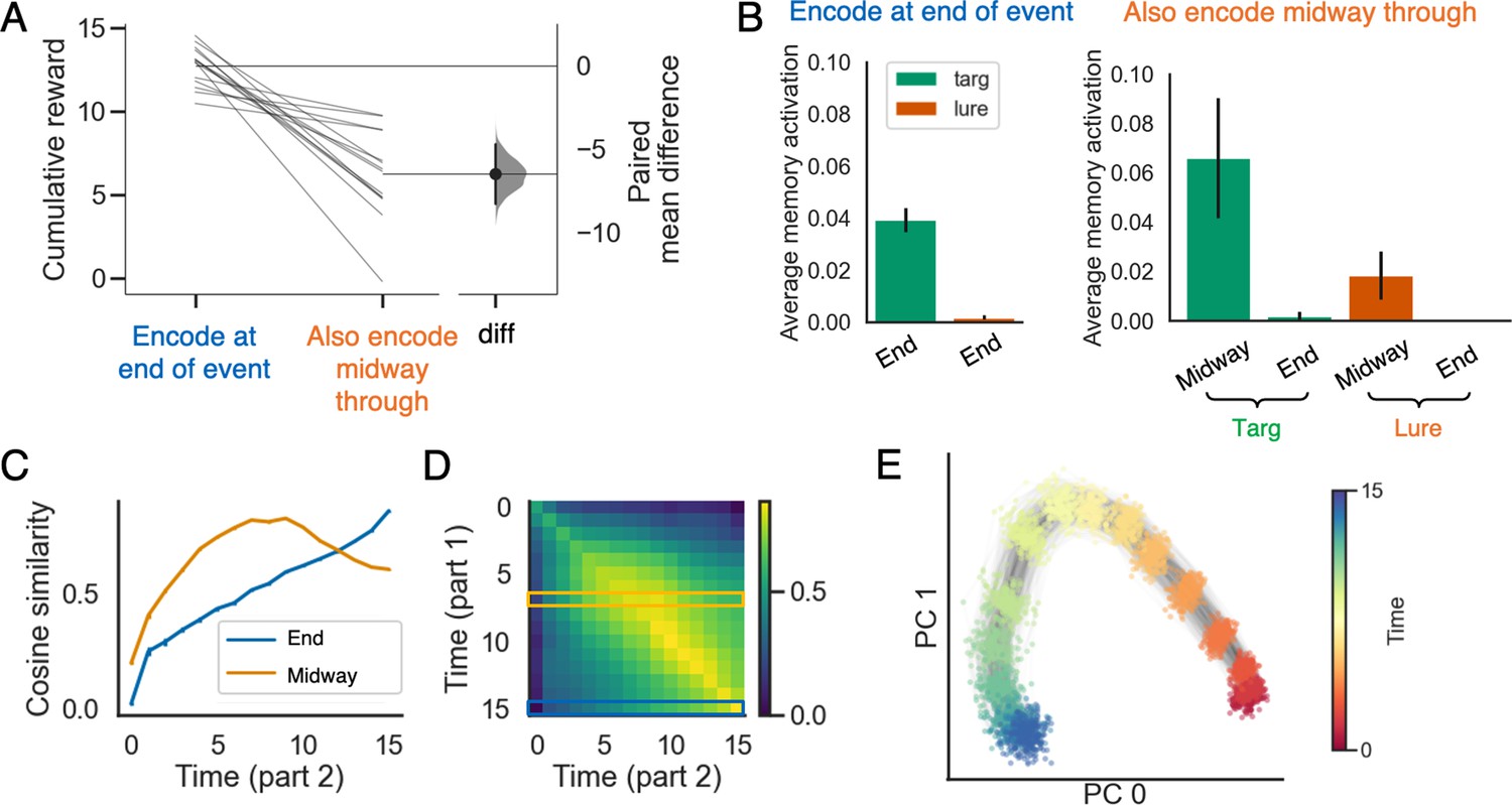
The advantage of selectively encoding episodic memories at the end of an event.
(A) Prediction performance is better for models that selectively encode at the end of each event, compared to models that encode at the end of each event and also midway through each event. (B) The model performs worse with midway-encoded memories because midway-encoded target memories are activated more strongly than end-encoded target memories, thereby blocking recall of the (more informative) end-encoded target memories, and also because midway-encoded lure memories are more strongly activated than end-encoded lure memories (see text for additional discussion). (C) The cosine similarity between working memory states during part 2 and memories formed midway through part 1 (in orange) or at the end of part 1 (in blue). The result indicates that the midway-encoded memory will dominate the end-encoded memory for most time points. (D) The time-point-to-time-point cosine similarity matrix between working memory states from part 1 versus part 2 in the no memory (NM) condition (part C depicts the orange and blue rows from this matrix). (E) PCA plot of working memory states as a function of time, for a large number of events. The plot shows that differences in time within events are represented much more strongly than differences across events. The errorbars indicate 1SE across 15 models.
Figure 5
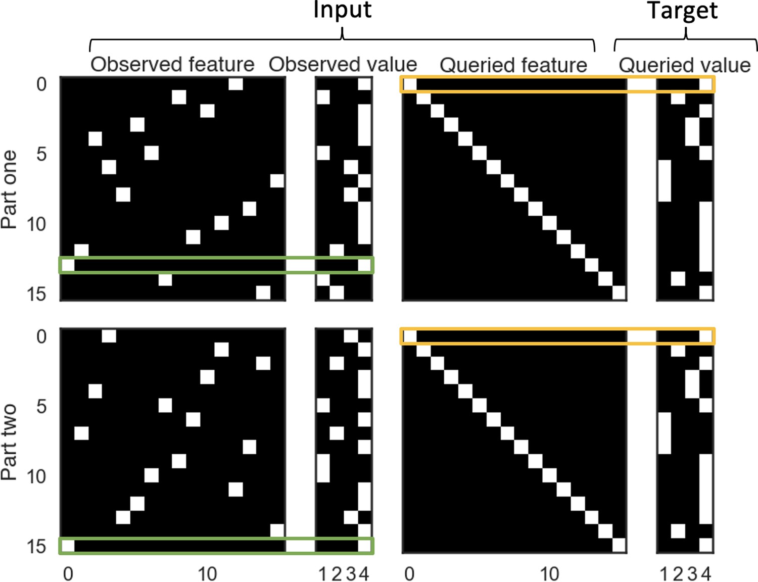
The stimulus representation for the event processing task.
In the event processing task, situation features are observed in different, random orders during part 1 and part 2, but queries about those features are presented in the same order during part 1 and part 2. The green boxes in panel A indicate time points where the model observed the value of the first feature (time point 13 during part 1, and time point 15 during part 2). The yellow boxes indicate time points where the model was queried about the value of the first feature (time point zero during both part 1 and part 2).
Appendix 1—figure 1
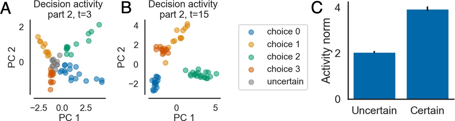
How certainty is represented in the model’s activity patterns.
Panels A and B show the neural activity patterns from the decision layer in the distant memory (DM) condition, projected onto the first two principal components. Each point corresponds to the pattern of neural activity for a trial at a particular time point. We colored the points based on the output (i.e., ‘choice‘) of the model, which represents the model’s belief about which state will happen next. Patterns that subsequently led to ‘don’t know‘ responses are colored in grey. Panel A shows an early time point with substantial uncertainty (a large number of ‘don’t know‘ responses). Panel B shows the last time point of this event, where the model has lower uncertainty. Panel C shows the average L2 norm of states that led to ‘don’t know‘ responses (uncertain) versus states that led to specific next-state predictions (certain); the errorbars indicate 1SE across 15 models. States corresponding to ‘don’t know‘ responses are clustered in the center of the activation space, with a lower L2 norm.
Appendix 2—figure 1
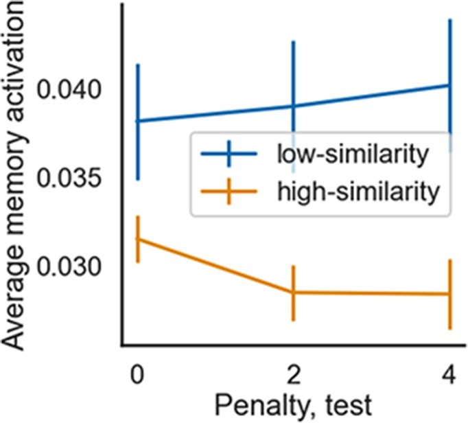
Memory activation during part 2 (averaged over time) in the DM condition, for models trained in low vs. high event-similarity environments and tested with penalty values that were low (penalty = 0), moderate (penalty = 2), or high (penalty = 4).
The model recalls less when similarity is high (vs. low), and this effect is larger for higher penalty values. The errorbars indicate 1SE across 15 models.
Appendix 3—figure 1
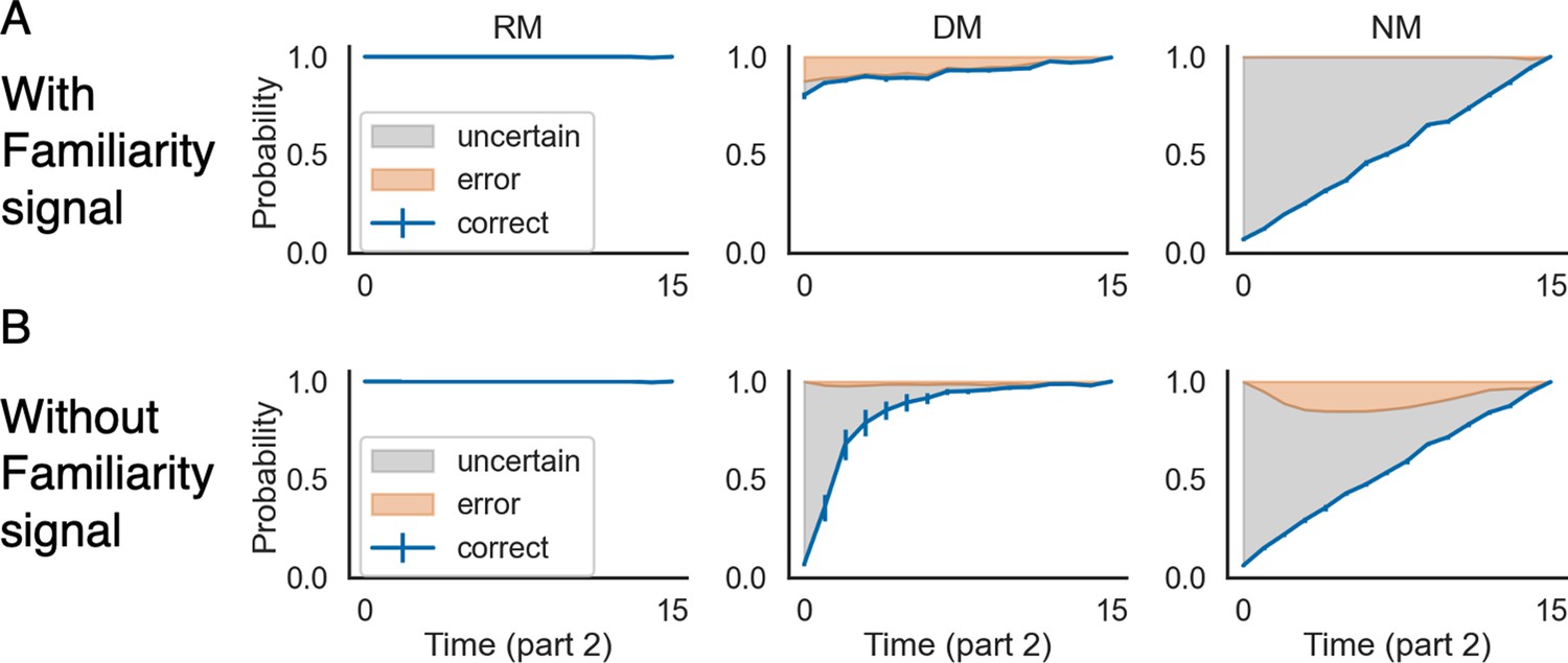
The familiarity signal can improve prediction.
Next-state prediction performance for models with (A) vs. without (B) access to the familiarity signal. With the familiarity signal (A), the model shows (1) higher levels of correct prediction in the DM condition, and (2) a reduced error rate in the NM condition. The errorbars indicate 1SE across 15 models.
Appendix 3—figure 2
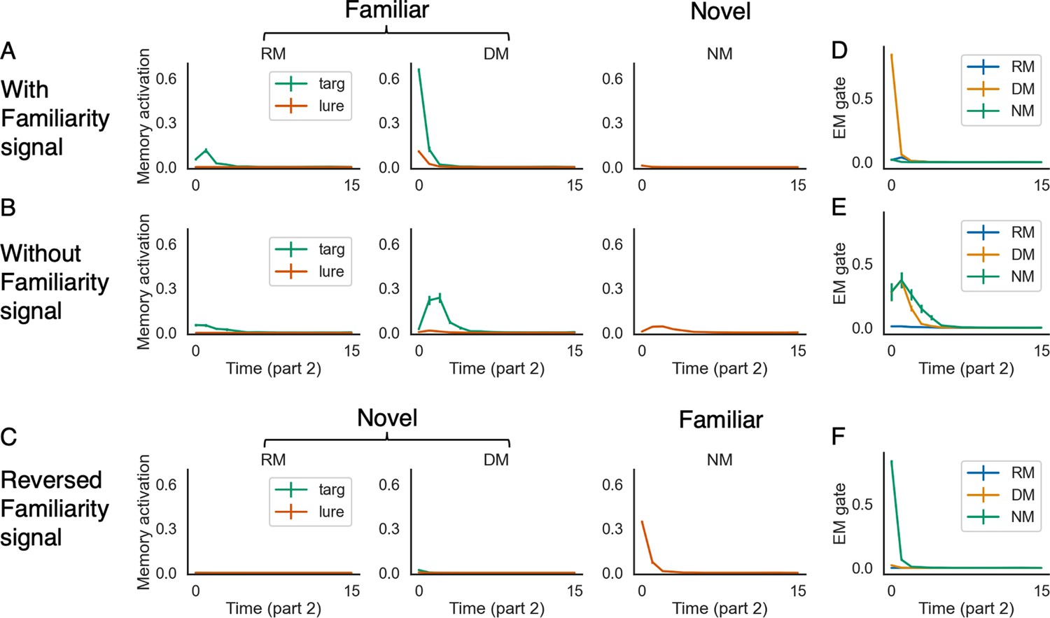
Episodic retrieval is modulated by familiarity.
This figure shows the memory activation and EM gate values over time for three conditions: (1) with the familiarity signal (A, D), (2) without the familiarity signal (B, E), and (3) with a reversed (opposite) familiarity signal at test (C, F). With the familiarity signal (A), the model shows higher levels of recall in the DM condition, and suppresses recall even further in the NM condition, compared to the model without the familiarity signal (B). This is due to the influence of the EM gate – the model with the familiarity signal retrieves immediately in the DM condition, and turns off episodic retrieval almost completely in the NM condition (D). Note also that levels of episodic retrieval in the RM condition stay low, even with the familiarity signal (see text for discussion). Finally, parts C and F show that reversing the familiarity signal at test suppresses recall in the DM condition and boosts recall in the NM condition. The errorbars indicate 1SE across 15 models.
Appendix 4—figure 1
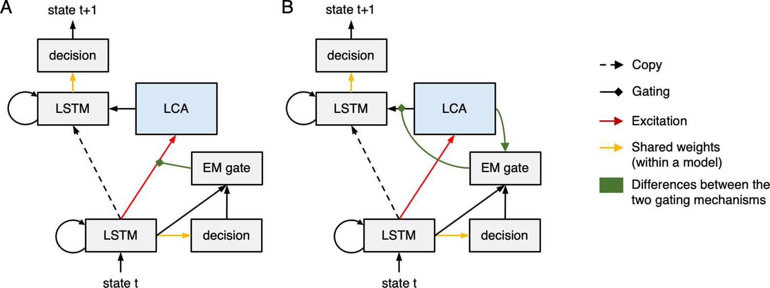
Unrolled network diagrams for the pre-gating (A) versus the post-gating (B) models.
The EM gate in the pre-gating model controls the degree to which stored memories are activated within the LCA module, but does not control the degree to which the activated memories are transmitted to the neocortex. By contrast, the EM gate in the post-gating model controls the degree to which activated memories in the LCA module are transmitted to the neocortex, but it does not control how these memory activations are computed in the first place.
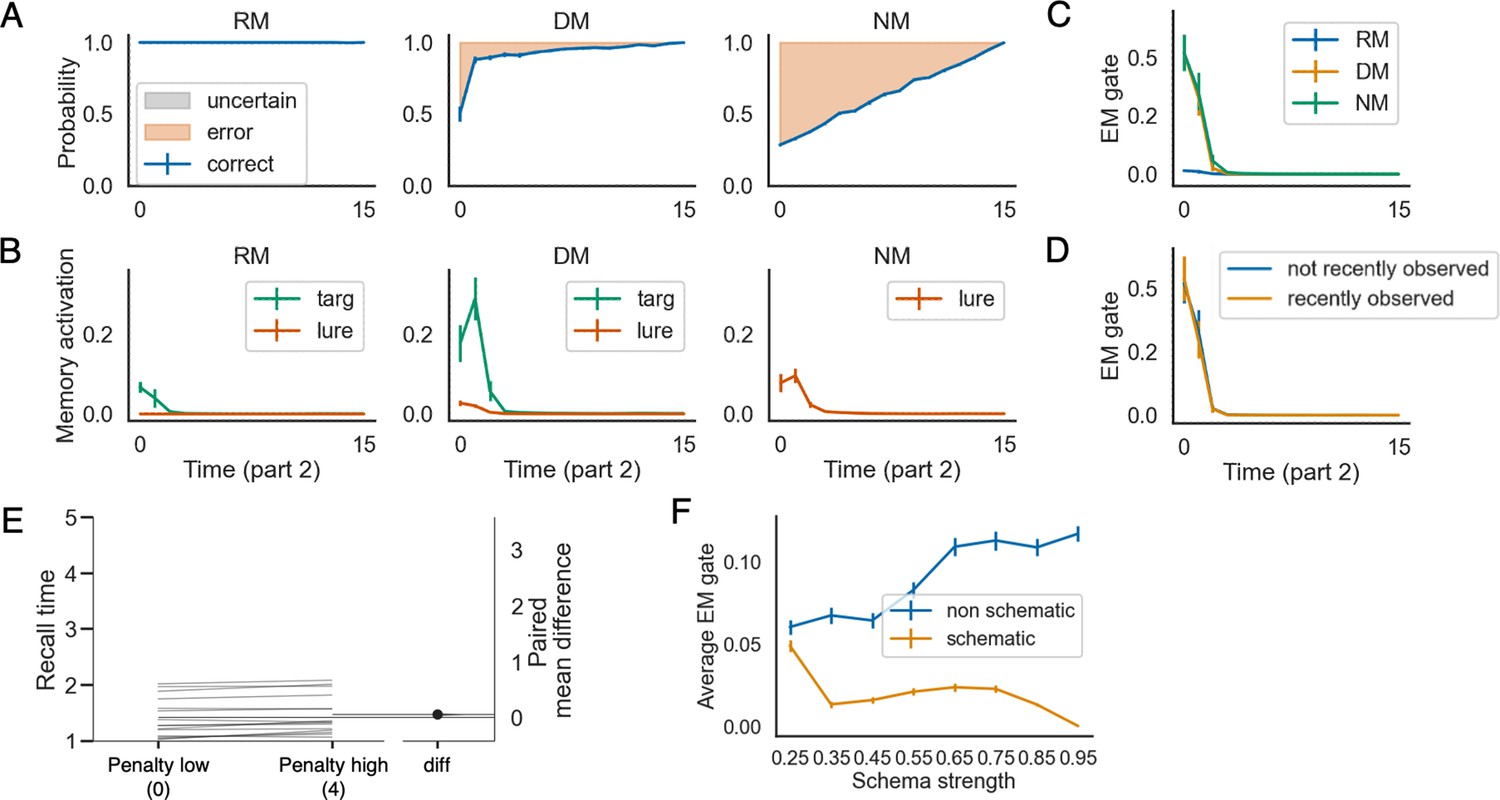
Appendix 4—figure 2
The post-gating model qualitatively replicates key results obtained from the pre-gating model (compare to Figures 3 and 4 in the main text).
See text in this appendix for discussion. The errorbars indicate 1SE across 15 models.
Appendix 5—figure 1
Results from a ‘no-RL‘ model that was trained in an entirely supervised fashion, without reinforcement learning and without the option of giving a ‘don’t know‘ response – compare to Figure 3 in the main text; see text in this appendix for discussion.
The errorbars indicate 1SE across 15 models.
Appendix 6—figure 1
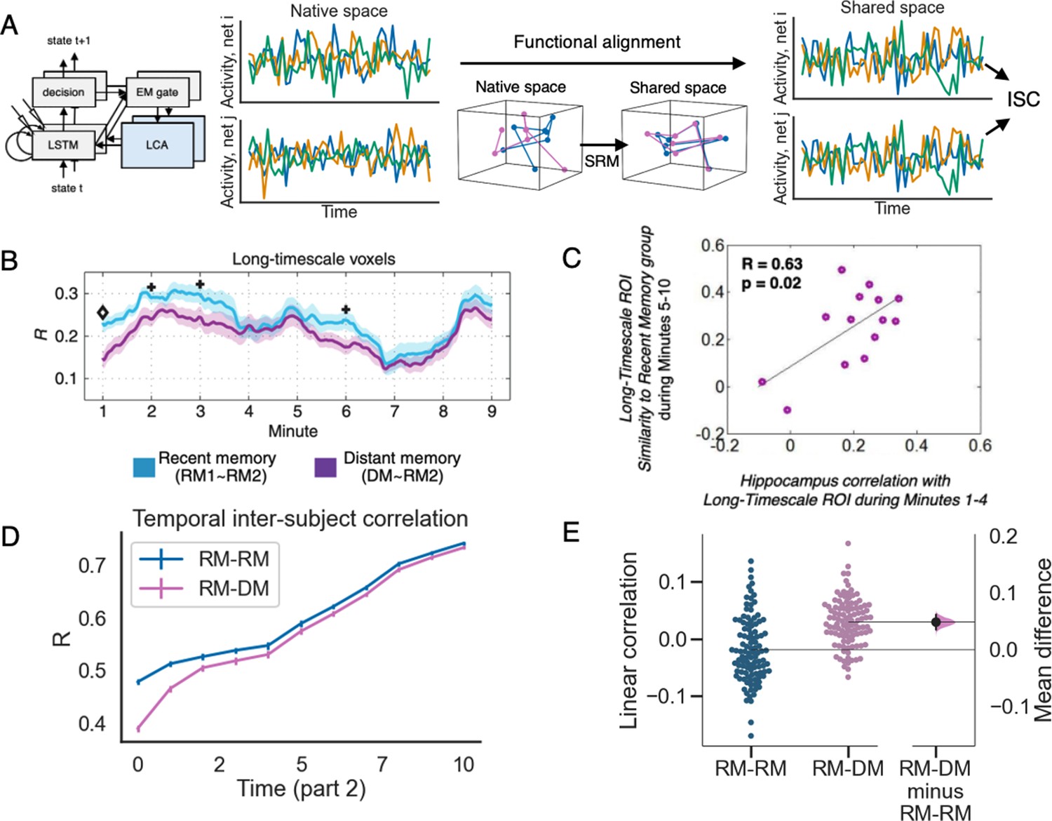
Simulating inter-subject correlation results from Chen et al., 2016.
(A) Illustration of how we computed inter-subject correlation (ISC) in the model (see text for details). (B and C) show the empirical results from Chen et al., 2016 (reprinted with permission) and (D and E) show model results. (B) The sliding-window temporal inter-subject correlation (ISC) over time, during part 2 of the movie. The recent memory ISC, or RM-RM ISC, was computed as the average ISC value between two non-overlapping subgroups of the RM participants. The distant memory ISC, or RM-DM ISC, was computed as the average ISC between one sub-group of RM participants and the DM participants. Initially, the RM-DM ISC was lower than RM-RM ISC, but as the movie unfolded, RM-DM ISC rose to the level of RM-RM ISC. (C) For the DM participants, the level of hippocampal-neocortical inter-subject functional connectivity at the beginning of part 2 of the movie (minutes 1–4) was correlated with the level of RM-DM ISC later on (minutes 5–10). (D) Sliding window temporal ISC in part 2 between the RM models (RM-RM) compared to ISC between the RM and DM models (RM-DM). The convergence between RM-DM ISC and RM-RM ISC shows that activity dynamics in the DM and the RM models become more similar over time (compare to part B of this figure). The errorbars indicate 1SE across 15 models. (E) The correlation in the model between memory activation at time and the change in ISC from time to time , for the first 10 time points in part 2. Each point is a subject-subject pair across the two conditions. The 95% bootstrap distribution on the side shows that the correlation between memory activation and the change in RM-DM ISC is significantly larger than the correlation between memory activation and the change in RM-RM ISC (see text for details).
© 2016, Oxford University Press Permissions. panel B is reprinted from Figure 6 Chen et al., 2016 by permission of Oxford University Press. It is not covered by the CC-BY 4.0 licence and further reproduction of this panel would need permission from the copyright holder
© 2016, Oxford University Press Permissions. panel C is reprinted from Figure S7 Chen et al., 2016, by permission of Oxford University Press. It is not covered by the CC-BY 4.0 licence and further reproduction of this panel would need permission from the copyright holder
Author response image 1
The model performed well in the task with repeating queries.
This figure can be compared with Figure 3 in the paper.
Author response image 2
Encoding midway through the event (in addition to encoding at the end) still hurts performance in the task with repeating queries.
This figure can be compared with Figure 4 in the paper.
Additional files
Download links
A two-part list of links to download the article, or parts of the article, in various formats.
Downloads (link to download the article as PDF)
Open citations (links to open the citations from this article in various online reference manager services)
Cite this article (links to download the citations from this article in formats compatible with various reference manager tools)
A neural network model of when to retrieve and encode episodic memories
eLife 11:e74445.
https://doi.org/10.7554/eLife.74445


