Functional brain reconfiguration during sustained pain
- Center for Neuroscience Imaging Research, Institute for Basic Science, Republic of Korea
- Department of Biomedical Engineering, Sungkyunkwan University, Republic of Korea
- Department of Intelligent Precision Healthcare Convergence, Sungkyunkwan University, Republic of Korea
Figures
Figure 1
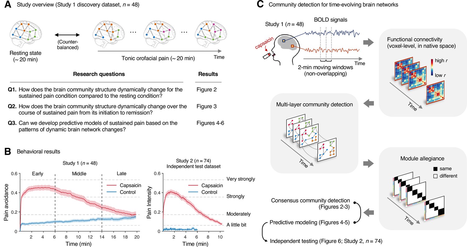
Study overview and behavioral results.
(A) Three main research questions of the current study. We aimed to answer the research questions by examining the time-varying patterns of functional brain network reconfiguration during 20 min of tonic orofacial pain experience and comparing them to the pain-free resting state. (B) Behavioral results. We asked participants to continuously report their pain in the scanner using either a pain avoidance rating scale (‘how much do you want to avoid this experience in the future?’) for Study 1 (‘discovery dataset,’ n = 48) or a pain intensity rating scale (‘how intense is your pain?’) for Study 2 (‘independent test dataset,’ n = 74). The anchors of the scale (the horizontal dashed lines) were based on a modified version of the general labeled magnitude scale (gLMS). The vertical dashed lines show how we define the early, middle, and late periods of sustained pain. The solid lines represent group mean ratings (red for capsaicin, and blue for control), and the shading represents standard errors of the mean (SEM). (C) The overview of main analyses. Voxel-level functional connectivity was estimated in the native space using 2 min moving windows and thresholded at 0.05 network density (see ‘Materials and methods’ for details). We identified the time-evolving network community structures from these suprathreshold connectivity matrices using the multilayer community detection method (Mucha et al., 2010), and calculated the module allegiance (Bassett et al., 2011). Using the module allegiance values as input features, we either identified group-level consensus community structures or conducted predictive modeling and tested the models on Study 2 independent test dataset (n = 74). Colored circles in the multilayer community detection and module allegiance analysis represent different community labels. Black- and white-colored boxes in the module allegiance matrices indicate whether or not the two different network nodes have the same community affiliation, respectively.
Figure 2
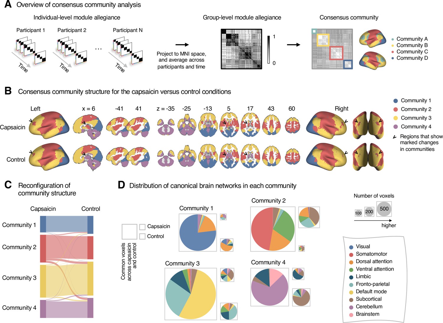
Reconfiguration of community structure for the sustained pain versus control conditions.
(A) Analysis overview. Individual module allegiance values computed in the native spaces were projected onto MNI space and averaged across all participants and all time-bins (i.e., ten bins) to yield a group-level module allegiance matrix. Then, we identified the group-level consensus community structures by decomposing the group-level module allegiance matrix into distinct modules using the Louvain community detection algorithm (Blondel et al., 2008). (B) Consensus community structure for the capsaicin versus control conditions. Community colors were determined based on the canonical network membership of the largest proportion of voxels across the two conditions. V-shaped arrows indicate the regions that showed marked changes in communities. (C) Voxel-wise changes in community assignments between the capsaicin and control conditions. (D) Proportions of 10 canonical brain networks—7 resting-state large-scale networks (Yeo et al., 2011), subcortical, cerebellum, and brainstem regions—for different communities. The large square on the left shows the network composition of the voxels common across the capsaicin and control conditions, and the squares on the upper and lower right represent the voxels uniquely assigned to the community for the capsaicin or control conditions, respectively. The sizes of the squares are proportional to the number of voxels.
Figure 3
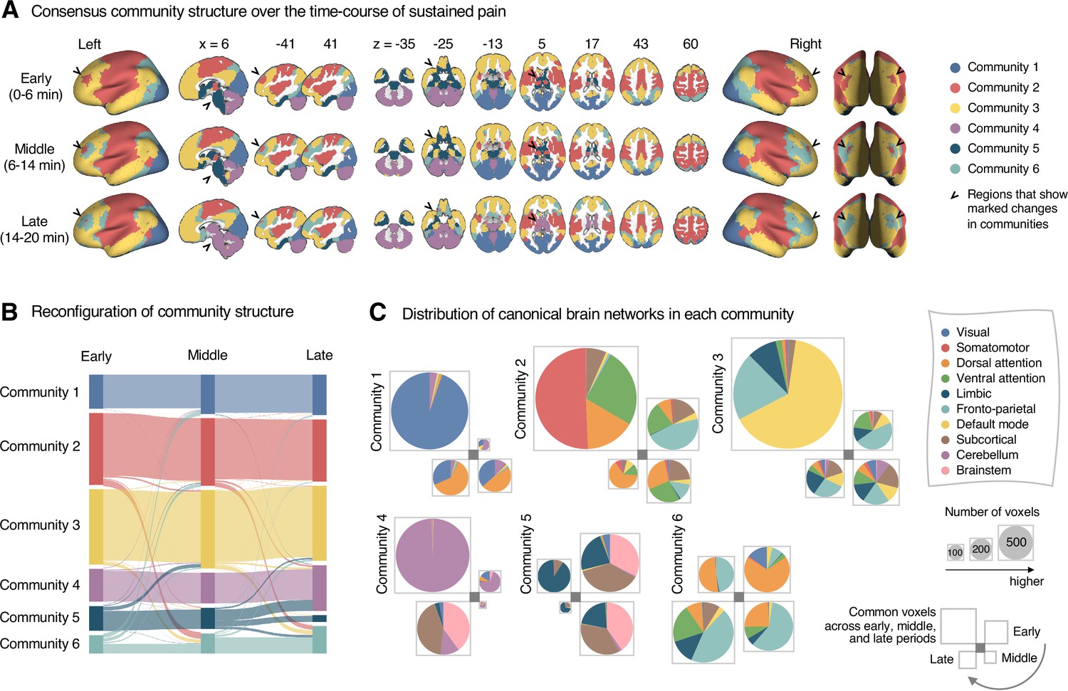
Reconfiguration of community structure over the time course of sustained pain experience.
(A) Consensus community structures of the early (0–6 min), middle (6–14 min), and late (14–20 min) periods of sustained pain. Colors indicate distinct community assignments and were determined based on the canonical network membership with the largest proportion of voxels across the periods. (B) Voxel-wise changes in community assignments from the early to late periods of pain. (C) Proportions of 10 canonical brain networks for different communities. The large square on the upper left shows the network composition of the voxels common across all periods, and the squares on the upper right, lower right, lower left represent the voxels of the early, middle, and late periods of pain after removing the common voxels, respectively. The sizes of the squares are proportional to the number of voxels.
Figure 4
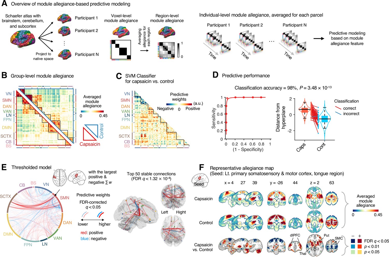
Module allegiance-based classifier for sustained pain versus resting.
(A) The analysis overview of the module allegiance-based predictive modeling. We first projected the whole-brain atlas onto an individual’s native brain space. We then averaged the voxel-level module allegiance values for each region to create region-level module allegiance matrices. These region-level module allegiance values were used to predict whether an individual was in pain or not. (B) Group-level module allegiance matrix. We averaged the region-level module allegiance matrices across all participants and all time-bins, and sorted the brain regions according to their canonical functional network membership. Lower and upper triangles represent the allegiance matrices of the capsaicin and control conditions, respectively. (C) Raw predictive weights of the support vector machine (SVM) classifier. (D) To obtain an unbiased estimate of the classifier’s classification performance, we conducted the forced-choice test with leave-one-participant-out cross-validation. Left: receiver-operating characteristics (ROC) curve. Right: cross-validated model responses for different conditions. Each line connecting dots represents an individual participant’s paired data (red: correct classification, blue: incorrect classification). p-Value was based on a binomial test, two-tailed. (E) Thresholded weights based on bootstrap tests with 10,000 iterations. Left: predictive weights thresholded at false discovery rate (FDR)-corrected q < 0.05 (which corresponds to uncorrected p<0.003), two-tailed. We indicated the brain region with the largest weighted degree centrality for positive and negative weights based on the thresholded model with the black arrow on the plot. Right: top 50 stable predictive weights (FDR q < 1.32 × 10⁻⁴, uncorrected p<1.91 × 10⁻⁷, two-tailed). (F) Seed-based allegiance map for the hub region that we identified in (E), left primary somatosensory and motor cortex (tongue region). The bottommost row shows the contrast map for the capsaicin versus control conditions, thresholded at t47 = 2.82, FDR q < 0.05 (uncorrected p<0.007), two-tailed, paired t-test. Put, putamen; dlPFC, dorsolateral prefrontal cortex; Thal, thalamus; SMC, somatomotor cortex; VN, visual network; SMN, somatomotor network; DAN, dorsal attention network; VAN, ventral attention network; LN, limbic network; FPN, frontoparietal network; DMN, default mode network; SCTX, subcortical regions; CB, cerebellum; BS, brainstem.
Figure 5
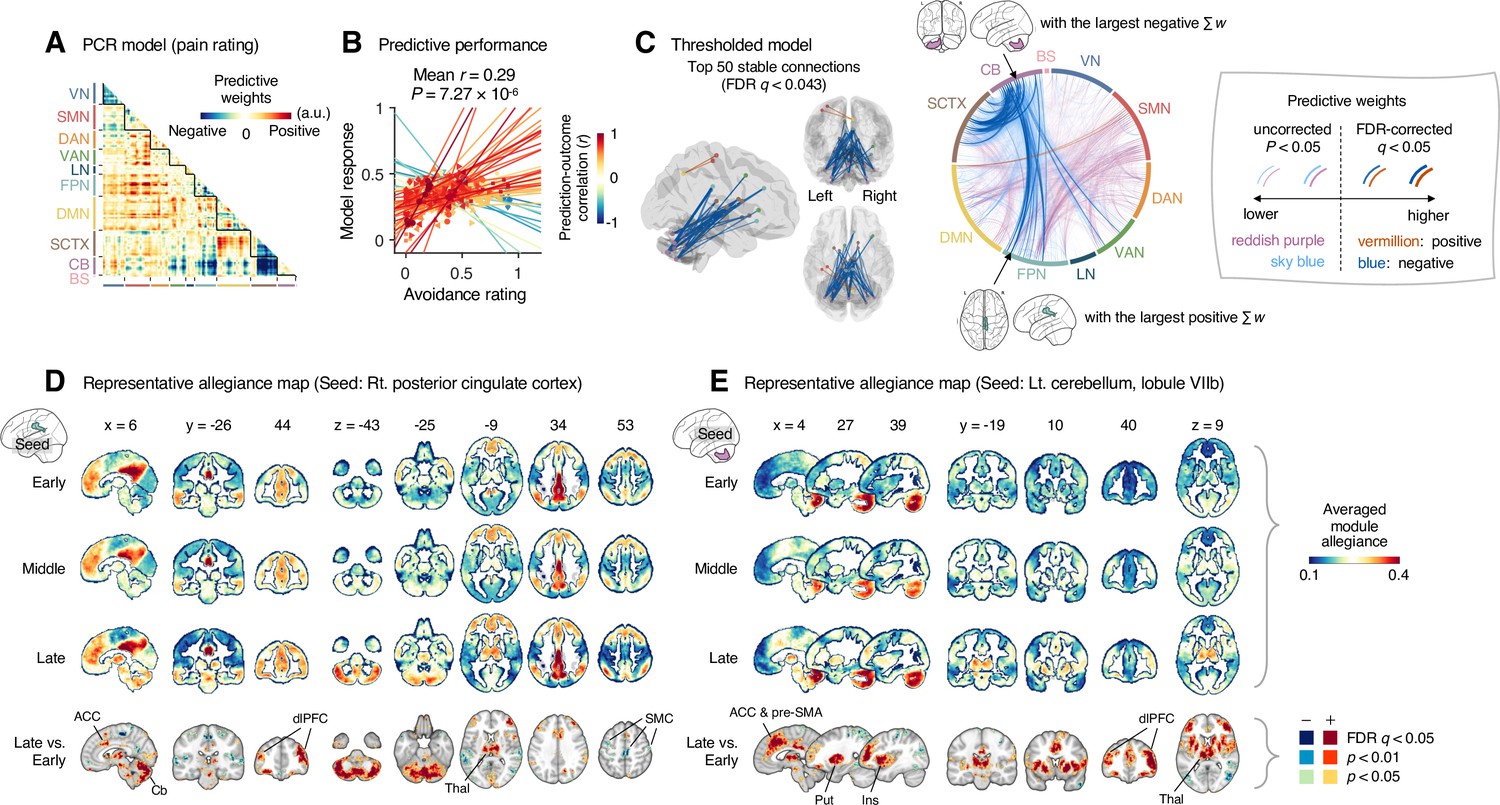
Module allegiance-based prediction model of pain rating.
(A) The raw predictive weights of the principal component regression (PCR) model based on region-level time-bin module allegiance matrices. (B) Actual versus predicted ratings. Each colored line (and symbol) represents individual participant’s ratings (10 time-bin average ratings per participant) during the capsaicin run (red: higher r; yellow: lower r; blue: r < 0). p-Value is based on bootstrap tests, two-tailed. (C) Thresholded weights based on bootstrap tests with 10,000 iterations. Left: top 50 stable predictive weights (false discovery rate [FDR]-corrected q < 0.043, which corresponds to uncorrected p<6.09 × 10⁻⁵, two-tailed). Right: FDR q < 0.05 (which corresponds to uncorrected p<9.24 × 10⁻⁵, vermillion and blue colors) or uncorrected p<0.05 (reddish purple and sky blue), two-tailed. The brain region with the largest weighted degree centrality separately for positive and negative weights is indicated with the black arrows. (D, E) Seed-based allegiance maps for the hub regions across different periods of sustained pain. The right posterior cingulate cortex (PCC) and left cerebellum lobule VIIb were identified as hub regions for the positive and negative weights, respectively. The bottommost row shows the contrast map for the late versus early periods, thresholded at t47 = 3.13 (D) and 3.22 (E), FDR q < 0.05 (which corresponds to uncorrected p<0.003 [D] and 0.002 [E]), two-tailed, paired t-test. ACC, anterior cingulate cortex; Cb, cerebellum; dlPFC, dorsolateral prefrontal cortex; Thal, thalamus; SMC, somatomotor cortex; pre-SMA, pre-supplementary motor area; Put, putamen; Ins, insula; VN, visual network; SMN, somatomotor network; DAN, dorsal attention network; VAN, ventral attention network; LN, limbic network; FPN, frontoparietal network; DMN, default mode network; SCTX, subcortical regions; CB, cerebellum; BS, brainstem.
Figure 6
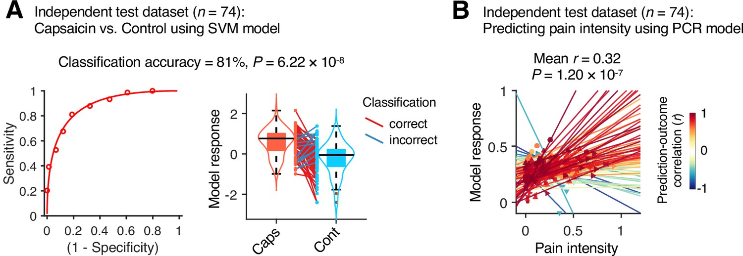
Model performance on an independent test dataset.
To provide unbiased estimates of prediction performance and test the generalizability of the module allegiance-based predictive models, we tested the support vector machine (SVM) and principal component regression (PCR) models on an independent test dataset (Study 2, n = 74). (A) We conducted a forced-choice test to compare the model responses for the capsaicin versus control conditions. Left: receiver-operating characteristics (ROC) curve. Right: model responses for different conditions. Each line connecting dots represents an individual participant’s paired data (red: correct classification; blue: incorrect classification). p-Value was based on a binomial test, two-tailed. (B) Actual versus predicted ratings. Each colored line (and symbol) represents individual participant’s ratings during the capsaicin run (red: higher r; yellow: lower r; blue: r < 0). p-Value was based on bootstrap tests, two-tailed.
Figure 7
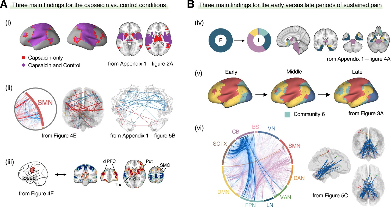
Graphical summary of the main findings.
We summarized the main findings to determine the main conclusion of this study. (A) Three main findings from the comparisons between the functional brain architectures of sustained pain (i.e., capsaicin) versus pain-free resting state (i.e., control) conditions (related to Q1 and Q3 in Figure 1A). During sustained pain, (i) an extended somatomotor-dominant community emerged. More specifically, the ventral part of somatomotor cortex regions (i.e., tongue area) was (ii) segregated from the original somatomotor-dominant community and (iii) integrated with the subcortical (e.g., basal ganglia, thalamus) and frontoparietal (e.g., dorsolateral prefrontal cortex) regions during sustained pain. (B) Three main findings from the comparisons between the early versus late periods of sustained pain (related to Q2 and Q3 in Figure 1A). (iv) In the early period, the brainstem was connected to the limbic brain regions including hippocampus, amygdala, parahippocampal gyrus, and temporal pole (c.f., the spino-brachio-amygdaloid circuit). (v) In the late period, the frontoparietal regions were dissociated from the extended somatomotor-dominant community and formed their own community. (vi) The cerebellar connections to the subcortical and frontoparietal regions were predictive of pain decrease.
Appendix 1—figure 1

Avoidance rating in Study 1.
(A) Participants reported their subjective ratings of avoidance continuously throughout the scan by moving the yellow-colored rating bar on the rating scale (gray triangle). The rating question was “how much do you want to avoid this experience in the future?” During the scan, we showed only the two extreme descriptors (i.e., ‘Not at all’ and ‘Most’) on the screen. (B) To enhance the reliability, we provided a detailed explanation of the locations and meaning of the anchors before the scan. The anchors included ‘Not at all,’ ‘A little bit,’ ‘Moderately,’ ‘Strongly,’ ‘Very strongly,’ and ‘Most.’ These anchors were not displayed during the scan.
Appendix 1—figure 2
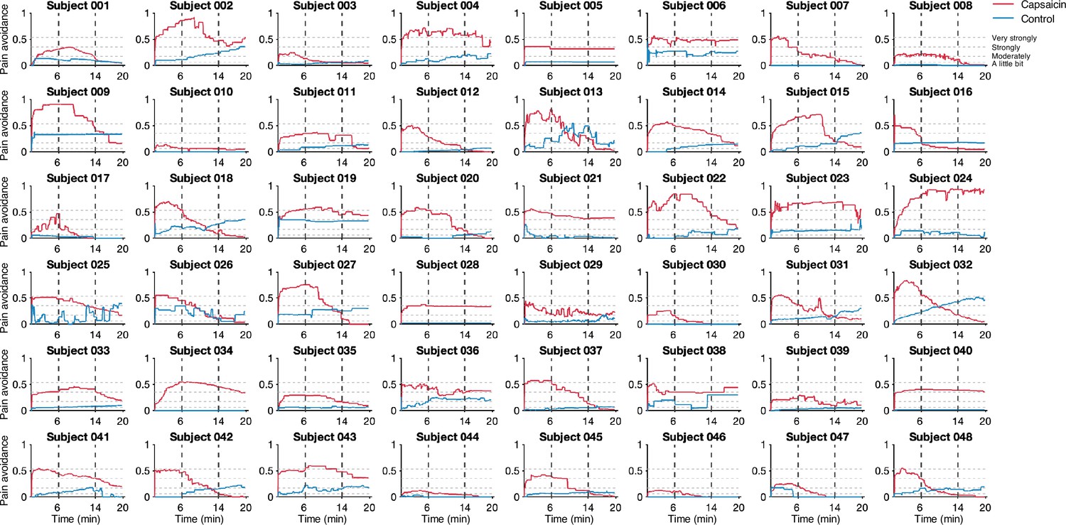
Pain avoidance ratings of individual participants.
These plots show the pain avoidance ratings of 48 participants from Study 1. The horizontal dashed lines indicate the anchors of the general labeled magnitude scale (gLMS). The vertical dashed lines show the time boundaries for the early, middle, and late periods of sustained pain. The red and blue solid lines show the pain avoidance ratings (red for the capsaicin run and blue for the control run).
Appendix 1—figure 3
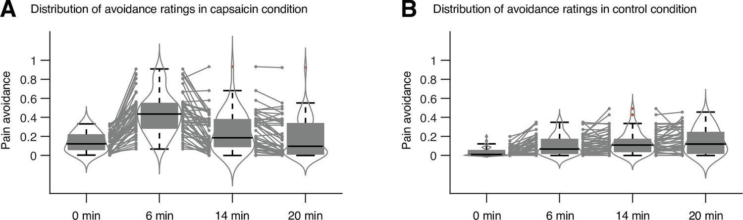
Distribution of avoidance ratings in Study 1.
We used the violin and box plots to show the distributions of the avoidance ratings, for the timepoints of 0 min, 6 min, 14 min, and 20 min. For each timepoint, 10 s time window was applied for averaging the ratings. The box was bounded by the first and third quartiles, and the whiskers stretched to the greatest and lowest values within median ± 1.5 interquartile range. The red dots outside of the whiskers were marked as outliers. Each gray line between gray dots represents each individual participant’s paired data.
Appendix 1—figure 4
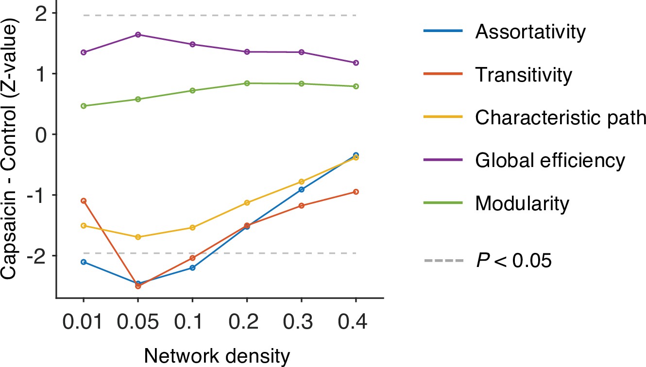
Global-level network attributes.
We compared the five global-level network attributes (i.e., assortativity, transitivity, characteristics path, global efficiency, and modularity) of the capsaicin and control conditions (z-values from paired z-test) across different levels of network density. Note that the overall differences of network attributes between the capsaicin versus control conditions were maximal at the network density of 0.05. All network attributes were measured from the binarized static connectivity matrices (for details, see ‘Materials and methods’).
Appendix 1—figure 5
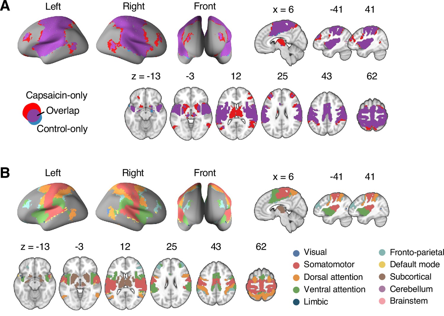
Reconfiguration of the consensus Community 2.
(A) We compared the spatial distributions of the consensus Community 2 (i.e., the somatomotor dominant community) of the capsaicin and control conditions. The purple regions show the overlap between the two conditions, and the red and blue regions show the unique regions for the capsaicin and control conditions, respectively. Blue region was comparatively small, indicating that the somatomotor community mainly expanded primarily during the capsaicin condition compared to the control condition. (B) The spatial distribution of the 10 canonical brain networks within the consensus Community 2. The expansion of Community 2 during the capsaicin condition (red regions in [A]) was mainly driven by the brain voxels within the frontoparietal network (e.g., dorsolateral prefrontal cortex and inferior parietal cortex) and the subcortical regions (e.g., thalamus and basal ganglia).
Appendix 1—figure 6
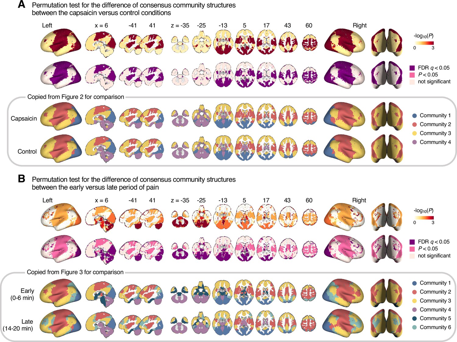
Permutation tests for the community structure changes.
We examined the regional differences in community structures between (A) the capsaicin versus control or (B) the early versus late period of pain. To quantitatively compare the group-level consensus community structures between the capsaicin versus control conditions and the early versus late periods, we first obtained a seed-based module allegiance map for each voxel (i.e., using each voxel as a seed). Then, we calculated a correlation coefficient of the module allegiance values between two different conditions for each voxel. This correlation coefficient can serve as an estimate of the voxel-level similarity of the consensus community profile. Because module allegiance is a binary variable, these correlation values are Phi coefficients (φ). To calculate the statistical significance of the Phi coefficient, we conducted permutation tests, in which we randomly shuffled the condition labels in each participant and obtained the group-level consensus community structure for each shuffled condition. Then, we calculated the voxel-level correlations of the module allegiance values between the two shuffled conditions. We repeated this procedure 1000 times to generate the null distribution of the Phi coefficients, and calculated the proportion of null samples that have a smaller Phi coefficient (i.e., a more dissimilar regional community structure) than the nonshuffled original data, which is the p-value, one-tailed. First row: -log10p values from the permutation tests. Second row: thresholded maps based on the p-values from the permutation tests. Colored as purple for false discovery rate (FDR)-corrected q < 0.05, pink for uncorrected p<0.05, and pale pink for nonsignificance. Third and last row: Group-level consensus community structures from Figures 2 and 3.
Appendix 1—figure 7
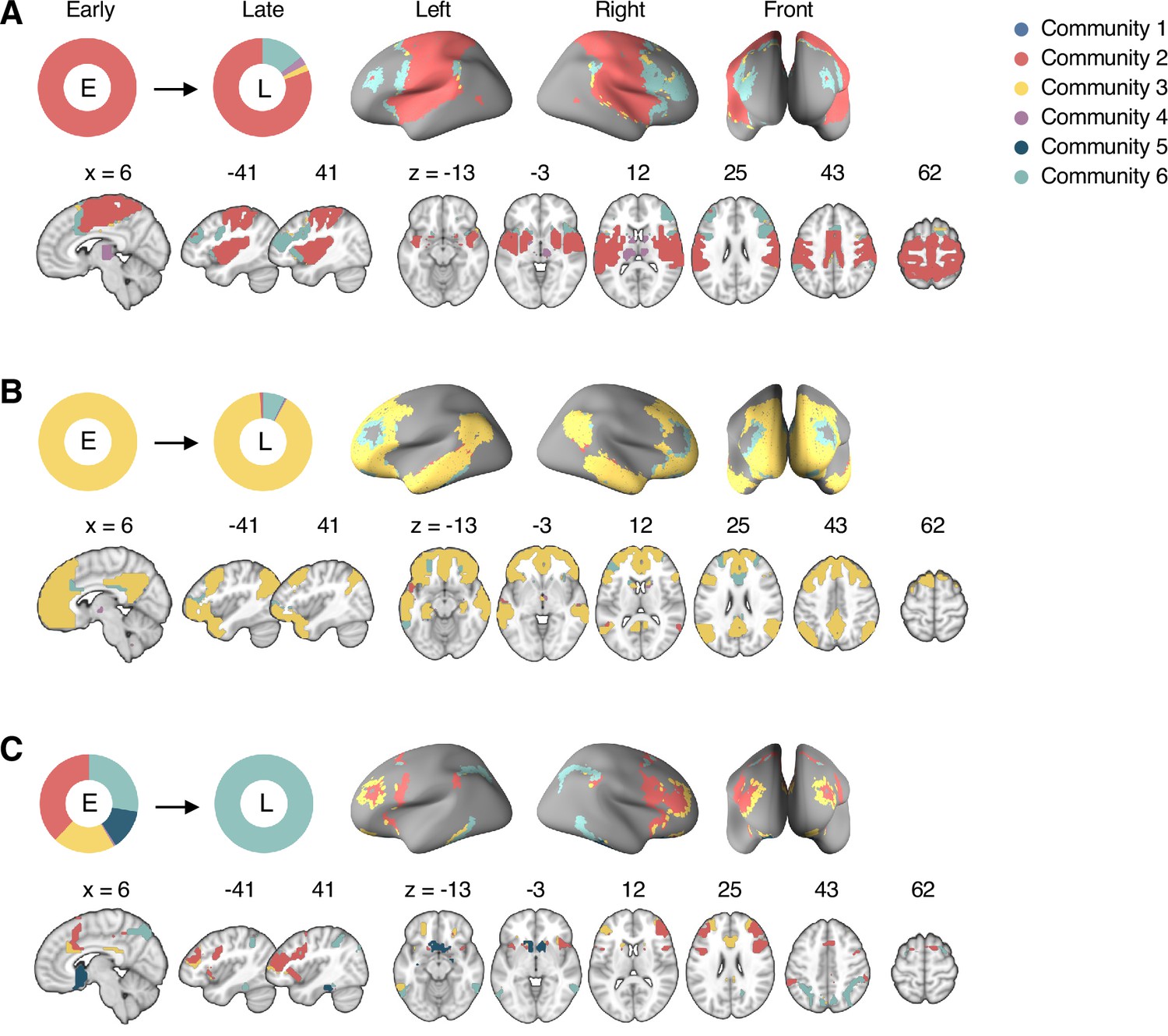
Reconfiguration of the consensus communities 2, 3, and 6.
The reconfiguration pattern of the community assignments of the brain voxels that were assigned to (A) the consensus Community 2 (somatomotor network dominant community) in the early period of sustained pain, (B) the consensus Community 3 (default-mode network dominant community) in the early period of sustained pain, and (C) the consensus Community 6 (frontoparietal network dominant community) in the late period of sustained pain. E, early; L, late.
Appendix 1—figure 8

Reconfiguration of the consensus communities 4 and 5.
The reconfiguration pattern of the community assignments of the brain voxels that were assigned to (A) the consensus Community 5 (limbic network dominant community) in the early period of sustained pain, and (B) the consensus Community 4 (cerebellum-dominant community) in the late period of sustained pain. E, early; L, late.
Appendix 1—figure 9
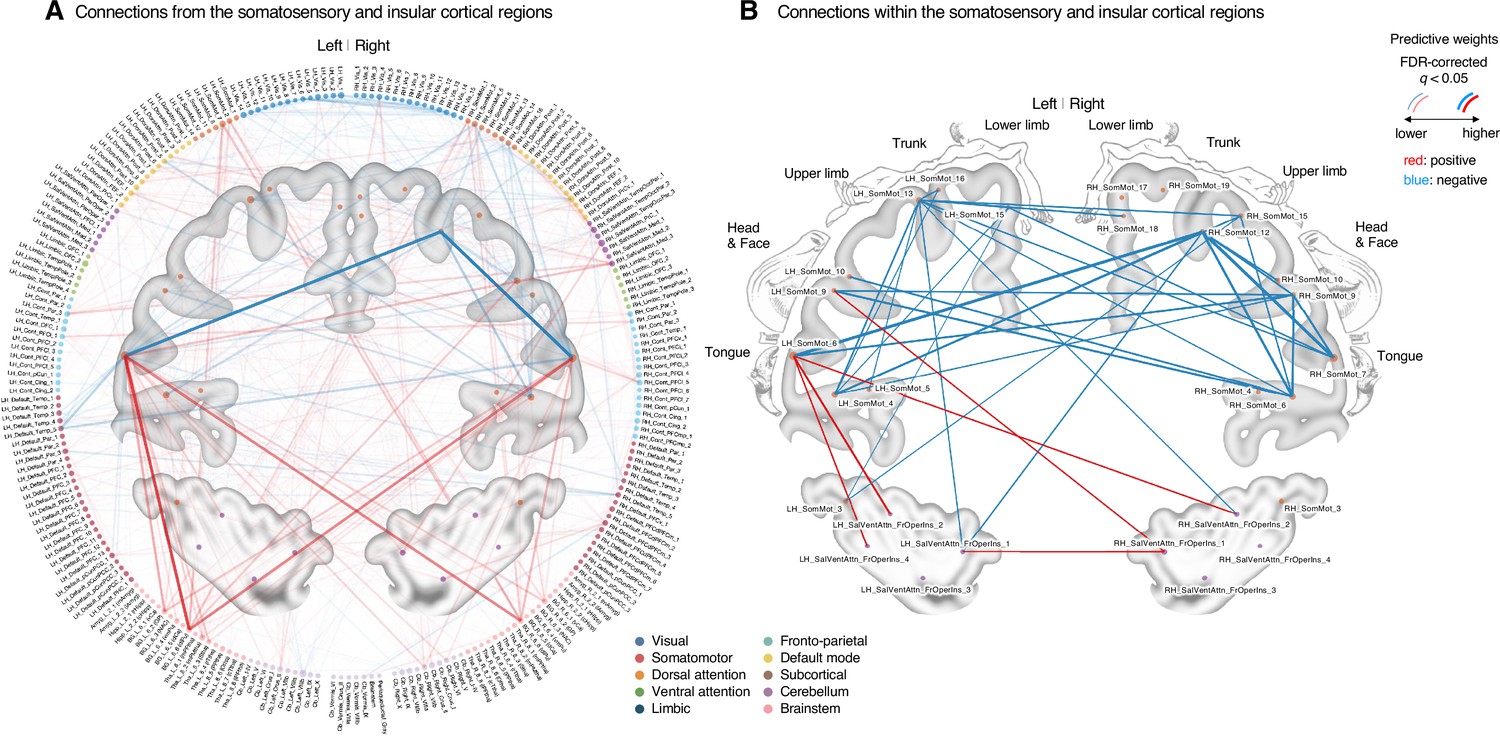
Classifier weights of the somatosensory and insular cortical regions.
(A) Thresholded connections (false discovery rate [FDR] q < 0.05, which corresponds to uncorrected p<0.003, two-tailed, bootstrap test with 10,000 iterations) showing the predictive weights between the somatosensory and insular cortical regions and the other remaining whole brain regions. Line thickness and transparency indicate the absolute magnitude of predictive weights. There were strong negative weights within the somatosensory cortical regions and strong positive weights between the tongue primary somatosensory regions and subcortical regions (e.g., basal ganglia). (B) Thresholded connections (FDR q < 0.05, which corresponds to uncorrected p<0.003, two-tailed, bootstrap test with 10,000 iterations) showing the predictive weights between the primary and secondary somatosensory and insular cortical regions. Line thickness indicates the absolute magnitude of the predictive weights. Note that the location of the nodes on the brain map may not reflect the exact center coordinates of the regions-of-interests, though we marked them on the closest locations on the map. The somatosensory homunculus (modified from Fig 17 in Penfield and Rasmussen, 1950, p.44) represents the overall somatotopic gradients.
Appendix 1—figure 10
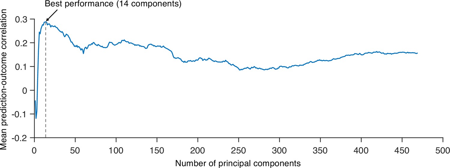
Predictive performances across different numbers of principal components (PCs).
We tested principal component regression (PCR) with a different number of PCs to find the best model to predict the within-individual variation of sustained pain ratings and calculated the mean correlation between actual and predicted pain ratings (10 ratings). Predictive performances were based on leave-one-subject-out cross-validation. The best model used 14 PCs for prediction.
Appendix 1—figure 11
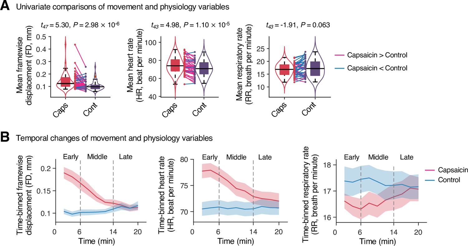
Head movement and physiology variables in Study 1.
(A) Comparisons of head motion (framewise displacement) and physiological measures (heart and respiratory rate) between the capsaicin versus control conditions. For significance testing, we conducted paired t-tests. (B) Temporal changes of head motion and physiology variables. Data were divided into 10 time-bins (2 min per bin). The vertical dashed lines show how we define the early, middle, and late periods of sustained pain. The solid lines represent group mean ratings (red for capsaicin, and blue for control), and the shading represents standard errors of the mean (SEM). Note that we needed to exclude four participants’ data due to technical issues with the physiological data acquisition.
Appendix 1—figure 12
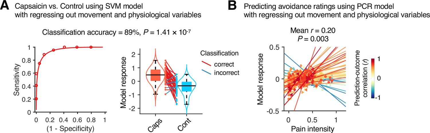
Prediction performance after controlling for head motion and physiological variables.
To examine whether head motion and physiology responses influenced the predictive model performance, we regressed out the framewise displacement (FD), heart rate (HR), and respiratory rate (RR) from the cross-validated model predictions in Study 1 (n = 44). (A) A forced-choice test to compare the model responses of the support vector machine (SVM) model for the capsaicin versus control conditions after regressing out the mean FD, HR, and RR. For regression, all the conditions and participants were concatenated as we trained the original SVM model. Left: receiver-operating characteristics (ROC) curve. Right: model responses for different conditions. Each line connecting dots represents an individual participant’s paired data (red: correct classification; blue: incorrect classification). p-Value was based on a binomial test, two-tailed. (B) Actual versus predicted values of the principal component regression (PCR) model after regressing out the 10-binned (2 min per bin) FD, HR, and RR. For regression, all the time-bins and participants were concatenated as we trained the original PCR model. Each colored line (and symbol) represents individual participant’s ratings during the capsaicin run (red: higher r; yellow: lower r; blue: r < 0). p-Value was based on bootstrap tests, two-tailed.
Appendix 1—figure 13
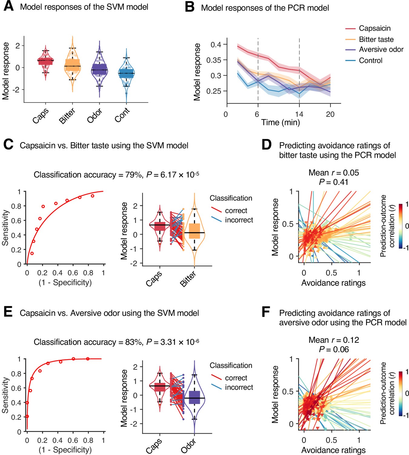
Specificity test results.
We tested the module allegiance-based support vector machine (SVM) and principal component regression (PCR) models of pain on the bitter taste (quinine) or aversive odor (fermented skate) conditions in Study 1 (n = 48) to examine the specificity of the models, using leave-one-participant-out cross-validation. (A, B) Model responses of the SVM model (A) and the PCR model (B) for capsaicin, bitter taste, aversive odor, and control conditions. The solid lines and shading in (B) represent the group mean ratings and standard errors of the mean (SEM), respectively. (C, E) Forced-choice test results of comparing the model responses for the capsaicin versus bitter taste (C) or aversive odor (E) conditions. Left: receiver-operating characteristics (ROC) curve. Right: model responses for different conditions. Each line connecting dots represents an individual participant’s paired data (red: correct classification; blue: incorrect classification). p-Values were based on a binomial test, two-tailed. (D, F) Actual versus predicted ratings. Each colored line (and symbol) represents individual participant’s ratings during the bitter taste run (D) or aversive odor run (F) (red: higher r; yellow: lower r; blue: r < 0). p-Value was based on bootstrap tests, two-tailed.
Author response image 1
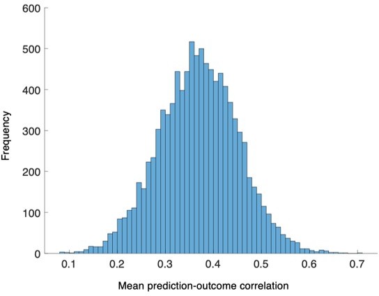
The distribution of the bootstrapped prediction-outcome correlations.
We conducted bootstrap tests to examine whether the distribution of within-individual prediction-outcome correlation coefficients of the PCR model were significantly different from zero for Study 1. The distribution of correlation coefficients met normality assumption, P = 0.27, Lilliefors test, two-tailed.
Tables
Appendix 1—table 1
Top 50 stable connections of the classification model.
| Rank | Weights | ROI names | MNI coordinates |
|---|---|---|---|
| Positive connections | |||
| #1 | 0.0222 | LH_SomMot_6 - BG_L_6_6 (dlPu) | (−56,–8,30) - (−28,–6,2) |
| #2 | 0.0200 | LH_SomMot_6 - BG_R_6_6 (dlPu) | (−56,–8,30) - (30,−4,2) |
| #3 | 0.0200 | RH_SomMot_7 - BG_L_6_6 (dlPu) | (58,−4,30) - (−28,–6,2) |
| #4 | 0.0181 | LH_SomMot_6 - BG_L_6_2 (GP) | (−56,–8,30) - (−22,–2,4) |
| #5 | 0.0170 | RH_SomMot_7 - BG_R_6_6 (dlPu) | (58,−4,30) - (30,−4,2) |
| #6 | 0.0162 | LH_SomMot_7 - BG_R_6_6 (dlPu) | (−48,–8,46) - (30,−4,2) |
| #7 | 0.0161 | RH_SomMot_7 - BG_L_6_2 (GP) | (58,−4,30) - (−22,–2,4) |
| #8 | 0.0160 | LH_SomMot_7 - BG_L_6_6 (dlPu) | (−48,–8,46) - (−28,–6,2) |
| #9 | 0.0156 | RH_DorsAttn_Post_9 - RH_SalVentAttn_TempOccPar_2 | (8,-56,62) - (60,−38,16) |
| #10 | 0.0154 | LH_SomMot_6 - BG_R_6_2 (GP) | (−56,–8,30) - (22,−2,4) |
| #11 | 0.0154 | RH_SalVentAttn_PrC_1 - RH_SalVentAttn_FrOperIns_3 | (50,4,40) - (36,24,4) |
| #12 | 0.0154 | LH_Cont_Par_3 - RH_SalVentAttn_Med_3 | (−46,–42,46) - (8,4,66) |
| #13 | 0.0153 | LH_SomMot_2 - BG_R_6_6 (dlPu) | (−52,–24,10) - (30,−4,2) |
| #14 | 0.0161 | LH_SomMot_6 - Cb_Right_VIIb | (−56,–8,30) - (−24,–58,–52) |
| #15 | 0.0160 | RH_SomMot_1 - BG_L_6_6 (dlPu) | (52,−14,6) - (−28,–6,2) |
| #16 | 0.0156 | LH_DorsAttn_FEF_1 - RH_Cont_PFCl_5 | (−32,–4,54) - (30,48,28) |
| #17 | 0.0154 | LH_SomMot_6 - Tha_L_8_2 (mPMtha) | (−56,–8,30) - (−18,–14,4) |
| #18 | 0.0154 | LH_SomMot_6 - Cb_Right_VI | (−56,–8,30) - (24,−58,−26) |
| #19 | 0.0153 | RH_SomMot_1 - BG_R_6_6 (dlPu) | (52,−14,6) - (30,−4,2) |
| #20 | 0.0139 | RH_SomMot_2 - BG_R_6_6 (dlPu) | (64,−24,8) - (30,−4,2) |
| #21 | 0.0133 | LH_SomMot_2 - BG_R_6_2 (GP) | (−52,–24,10) - (22,−2,4) |
| #22 | 0.0131 | RH_SomMot_2 - BG_R_6_2 (GP) | (64,−24,8) - (22,−2,4) |
| #23 | 0.0130 | RH_SomMot_7 - BG_R_6_2 (GP) | (58,−4,30) - (22,−2,4) |
| #24 | 0.0127 | LH_SomMot_7 - BG_L_6_2 (GP) | (−48,–8,46) - (−22,–2,4) |
| #25 | 0.0127 | LH_SomMot_6 - Cb_Left_VI | (−56,–8,30) - (−22,–58,–24) |
| #26 | 0.0125 | RH_SomMot_10 - BG_R_6_6 (dlPu) | (46,−12,48) - (30,−4,2) |
| #27 | 0.0118 | LH_SomMot_6 - Cb_Left_VIIb | (−56,–8,30) - (−26,–66,–50) |
| #28 | 0.0113 | LH_SomMot_6 - Tha_R_8_8 (lPFtha) | (−56,–8,30) - (12,−16,6) |
| #29 | 0.0112 | LH_SomMot_7 - BG_R_6_2 (GP) | (−48,–8,46) - (22,−2,4) |
| #30 | 0.0111 | LH_Vis_8 - Tha_L_8_2 (mPMtha) | (−48,–70,10) - (−18,–14,4) |
| #31 | 0.0104 | LH_SomMot_13 - LH_Default_PFC_7 | (−26,–38,68) - (–8,58,20) |
| #32 | 0.0104 | LH_Vis_8 - LH_Cont_Cing_1 | (−48,–70,10) - (−4,–28,26) |
| #33 | 0.0103 | RH_SomMot_2 - Tha_L_8_2 (mPMtha) | (64,−24,8) - (−18,–14,4) |
| #34 | 0.0095 | LH_SomMot_13 - LH_Default_PFC_2 | (−26,–38,68) - (−6,36,–10) |
| #35 | 0.0092 | LH_SomMot_7 - Cb_Right_VI | (−48,–8,46) - (24,−58,−26) |
| #36 | 0.0092 | LH_SomMot_13 - RH_Default_PFCdPFCm_1 | (−26,–38,68) - (4,36,−14) |
| #37 | 0.0077 | LH_Cont_Cing_1 - RH_Vis_5 | (−4,–28,26) - (48,−72,−6) |
| #38 | 0.0067 | LH_SomMot_13 - LH_Limbic_OFC_2 | (−26,–38,68) - (−10,36,–20) |
| Negative connections | |||
| #1 | –0.0235 | RH_SomMot_7 - RH_SomMot_12 | (58,−4,30) - (40,−24,58) |
| #2 | –0.0231 | LH_SomMot_6 - RH_SomMot_12 | (−56,–8,30) - (40,−24,58) |
| #3 | –0.0160 | LH_SomMot_4 - RH_SomMot_12 | (−54,–4,10) - (40,−24,58) |
| #4 | –0.0145 | RH_SomMot_6 - RH_SomMot_14 | (56,−12,14) - (32,−22,64) |
| #5 | –0.0143 | LH_SomMot_6 - LH_Default_Temp_3 | (−56,–8,30) - (−56,–6,–12) |
| #6 | –0.0141 | LH_SomMot_6 - LH_Default_Temp_4 | (−56,–8,30) - (−58,–30,–4) |
| #7 | –0.0135 | LH_SomMot_6 - LH_Default_pCunPCC_1 | (−56,–8,30) - (−12,–56,14) |
| #8 | –0.0124 | LH_SomMot_4 - LH_SomMot_13 | (−54,–4,10) - (−26,–38,68) |
| #9 | –0.0115 | LH_SomMot_4 - RH_SomMot_14 | (−54,–4,10) - (32,−22,64) |
| #10 | –0.0092 | RH_SalVentAttn_Med_1 - Cb_Left_VIIIb | (8,8,42) - (0,–64,–42) |
| #11 | –0.0084 | LH_SalVentAttn_FrOperIns_4 - Cb_Left_VIIIb | (–52,8,10) - (0,–64,–42) |
| #12 | –0.0083 | LH_SalVentAttn_Med_1 - Cb_Left_VIIIb | (–6,10,42) - (0,–64,–42) |
-
Top 50 stable connections based on bootstrap tests with 10,000 iterations (edge-level p<1.9 × 10⁻⁷, FDR q < 1.4 × 10⁻⁴).
-
FDR, false discovery rate; ROI, region of interest.
Appendix 1—table 2
Top 50 stable connections of the regression model.
| Rank | Weights | ROI names | MNI coordinates |
|---|---|---|---|
| Positive connections | |||
| #1 | 0.000496 | LH_SomMot_12 - RH_Default_pCunPCC_3 | (−32,–22,64) - (6,−58,44) |
| #2 | 0.000460 | LH_SomMot_10 - RH_Default_pCunPCC_3 | (−40,–26,58) - (6,−58,44) |
| Negative connections | |||
| #1 | –0.000768 | RH_Cont_Cing_1 - Cb_Left_Crus_II | (6,–26,30) - (−26,–74,–42) |
| #2 | –0.000756 | RH_Cont_Cing_1 - Cb_Left_Crus_I | (6,–26,30) - (−36,–68,–32) |
| #3 | –0.000743 | Tha_R_8_1 (mPFtha) - Cb_Vermis_VI | (8,–10,6) - (0,–70,–22) |
| #4 | –0.000711 | Tha_R_8_1 (mPFtha) - Cb_Vermis_VIIIa | (8,–10,6) - (26,–58,–54) |
| #5 | –0.000697 | RH_Cont_Cing_1 - Cb_Right_Crus_I | (6,–26,30) - (38,–68,–32) |
| #6 | –0.000695 | RH_Cont_Cing_1 - Cb_Vermis_IX | (6,–26,30) - (6,–54,–48) |
| #7 | –0.000694 | Tha_R_8_1 (mPFtha) - Cb_Left_VIIb | (8,–10,6) - (−26,–66,–50) |
| #8 | –0.000673 | RH_Cont_Cing_1 - Cb_Right_Crus_II | (6,–26,30) - (26,–76,–42) |
| #9 | –0.000662 | Tha_R_8_1 (mPFtha) - Cb_Left_Crus_I | (8,–10,6) - (−36,–68,–32) |
| #10 | –0.000655 | Tha_R_8_1 (mPFtha) - Cb_Vermis_IX | (8,–10,6) - (6,–54,–48) |
| #11 | –0.000655 | LH_Cont_Cing_1 - Cb_Left_Crus_I | (−4,–28,26) - (−36,–68,–32) |
| #12 | –0.000654 | RH_Cont_PFCmp_1 - Cb_Left_Crus_I | (8,30,28) - (−36,–68,–32) |
| #13 | –0.000652 | RH_Cont_PFCmp_1 - Cb_Left_Crus_II | (8,30,28) - (−26,–74,–42) |
| #14 | –0.000650 | Tha_R_8_1 (mPFtha) - Cb_Left_Crus_II | (8,-10,6) - (−26,–74,–42) |
| #15 | –0.000648 | LH_Cont_Cing_1 - Cb_Left_Crus_II | (−4,–28,26) - (−26,–74,–42) |
| #16 | –0.000647 | Tha_L_8_1 (mPFtha) - Cb_Vermis_VI | (−6,–12,6) - (0,–70,–22) |
| #17 | –0.000643 | LH_Cont_Cing_1 - Cb_Right_Crus_I | (−4,–28,26) - (38,–68,–32) |
| #18 | –0.000642 | Tha_R_8_1 (mPFtha) - Cb_Right_VIIb | (8,–10,6) - (−24,–58,–52) |
| #19 | –0.000626 | BG_R_6_1 (vCa) - Cb_Vermis_VI | (14,14,–2) - (0,–70,–22) |
| #20 | –0.000624 | LH_Cont_Cing_1 - Cb_Right_Crus_II | (−4,–28,26) - (26,–76,–42) |
| #21 | –0.000598 | Tha_R_8_1 (mPFtha) - Cb_Right_VI | (8,–10,6) - (24,–58,–26) |
| #22 | –0.000592 | Tha_R_8_1 (mPFtha) - Cb_Right_Crus_I | (8,–10,6) - (38,–68,–32) |
| #23 | –0.000578 | RH_SalVentAttn_FrOperIns_3 - Cb_Left_VIIb | (36,24,4) - (−26,–66,–50) |
| #24 | –0.000565 | LH_SalVentAttn_Med_1 - Cb_Left_VIIb | (–6,10,42) - (−26,–66,–50) |
| #25 | –0.000549 | Tha_L_8_7 (cTtha) - Cb_Left_Crus_I | (−10,–22,14) - (−36,–68,–32) |
| #26 | –0.000543 | Tha_L_8_7 (cTtha) - Cb_Left_VIIb | (−10,–22,14) - (−26,–66,–50) |
| #27 | –0.000538 | BG_L_6_5 (dCa) - Cb_Vermis_VIIIa | (–14,2,16) - (26,–58,-54) |
| #28 | –0.000532 | LH_SalVentAttn_Med_1 - Cb_Right_VIIb | (–6,10,42) - (−24,–58,–52) |
| #29 | –0.000530 | BG_L_6_5 (dCa) - Cb_Vermis_VI | (–14,2,16) - (0,–70,–22) |
| #30 | –0.000530 | Tha_L_8_7 (cTtha) - Cb_Left_Crus_II | (−10,–22,14) - (−26,–74,–42) |
| #31 | –0.000523 | BG_R_6_5 (dCa) - Cb_Left_Crus_I | (14,6,14) - (−36,–68,–32) |
| #32 | –0.000520 | BG_R_6_5 (dCa) - Cb_Left_VIIb | (14,6,14) - (−26,–66,–50) |
| #33 | –0.000519 | Tha_L_8_1 (mPFtha) - Cb_Left_Crus_I | (−6,–12,6) - (−36,–68,–32) |
| #34 | –0.000515 | BG_R_6_5 (dCa) - Cb_Left_Crus_II | (14,6,14) - (−26,–74,–42) |
| #35 | –0.000494 | BG_L_6_5 (dCa) - Cb_Left_VIIb | (–14,2,16) - (−26,–66,–50) |
| #36 | –0.000481 | BG_L_6_4 (vmPu) - Cb_Right_VI | (−22,6,–4) - (24,–58,-26) |
| #37 | –0.000477 | Tha_R_8_4 (rTtha) - Cb_Left_Crus_II | (2,–12,6) - (−26,–74,–42) |
| #38 | –0.000473 | Tha_R_8_4 (rTtha) - Cb_Left_Crus_I | (2,–12,6) - (−36,–68,–32) |
| #39 | –0.000470 | BG_L_6_5 (dCa) - Cb_Left_Crus_I | (–14,2,16) - (−36,–68,–32) |
| #40 | –0.000469 | BG_R_6_5 (dCa) - Cb_Right_Crus_I | (14,6,14) - (38,–68,–32) |
| #41 | –0.000454 | BG_R_6_5 (dCa) - Cb_Right_VIIb | (14,6,14) - (−24,–58,–52) |
| #42 | –0.000448 | BG_L_6_5 (dCa) - Cb_Left_Crus_II | (–14,2,16) - (−26,–74,–42) |
| #43 | –0.000444 | RH_Cont_PFCv_1 - Cb_Left_Crus_II | (34,22,–8) - (−26,–74,–42) |
| #44 | –0.000443 | BG_L_6_5 (dCa) - Cb_Right_VIIb | (–14,2,16) - (−24,–58,–52) |
| #45 | –0.000434 | BG_R_6_5 (dCa) - Cb_Right_VI | (14,6,14) - (24,–58,–26) |
| #46 | –0.000421 | BG_L_6_5 (dCa) - Cb_Right_Crus_I | (–14,2,16) - (38,–68,–32) |
| #47 | –0.000405 | BG_L_6_5 (dCa) - Cb_Right_VI | (–14,2,16) - (24,–58,–26) |
| #48 | –0.000393 | BG_L_6_5 (dCa) - Cb_Left_VI | (–14,2,16) - (−22,–58,–24) |
-
Top 50 stable connections based on bootstrap tests with 10,000 iterations (edge-level p<6.1 × 10⁻⁵, FDR q < 0.043).
-
FDR, false discovery rate; ROI, region of interest.
Additional files
Download links
A two-part list of links to download the article, or parts of the article, in various formats.
Downloads (link to download the article as PDF)
Open citations (links to open the citations from this article in various online reference manager services)
Cite this article (links to download the citations from this article in formats compatible with various reference manager tools)
Functional brain reconfiguration during sustained pain
eLife 11:e74463.
https://doi.org/10.7554/eLife.74463


