Neural excursions from manifold structure explain patterns of learning during human sensorimotor adaptation
- Centre for Neuroscience Studies, Queen's University, Canada
- Department of Psychology, Queen's University, Canada
- School of Psychology, Centre for Computational Neuroscience and Cognitive Robotics, University of Birmingham, United Kingdom
- Department of Biomedical and Molecular Sciences, Queen's University, Canada
Figures
Figure 1
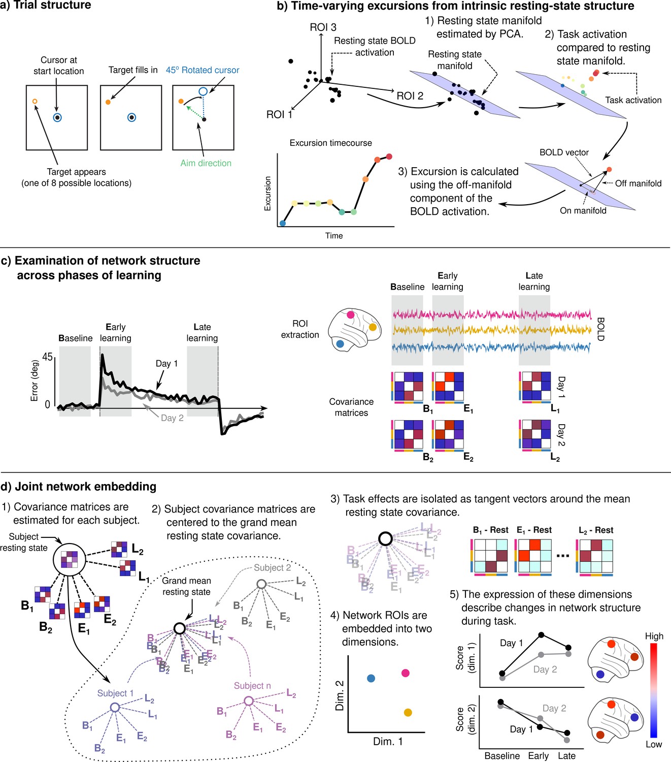
Adaptation task and analysis approach for the neural data.
(a) Visuomotor rotation (VMR) trial structure. Subjects used a force-sensitive joystick to move a cursor to a cued target location. On rotation trials, the mapping between aim and cursor direction was rotated clockwise by 45°. (b) We studied the degree to which learning is associated with the generation of novel patterns of neural activity by estimating resting-state manifolds for each subject, and then calculating the magnitude of the off-manifold component of the BOLD signal at each imaging volume during task. This measure, which we call excursion, provides a moment-by-moment index of functional reconfiguration of a brain network over the course of learning. (c) We studied functional network structure during baseline, early, and late learning on each day (mean subject learning curves shown on left over these epochs) by estimating covariance matrices from the mean BOLD signals extracted from cognitive and motor regions of interest (ROIs). (d) We isolated learning-related changes in functional network structure by centering subjects with respect to their resting-state network structure. We then jointly embedded networks estimated during each learning epoch into a common space in order to characterize changes in network structure over the time course of learning.
Figure 2

Clustering reveals three distinct groups of learners across days.
(a) (Top) Mean angle error during baseline, rotation, and washout on both days. Gray bands denote early and late rotation periods, and early washout. Colored bands denote standard errors. (Bottom) Early error on each day (mean error during the early learning window), as well as savings. (b) (Top) Variables used for clustering. (Bottom, from left) Dendrogram obtained by hierarchical complete linkage clustering on the distance for the above variables for each subject. Distance matrix displaying the distance between individual subjects’ clustering variables. The cluster solution was evaluated using the procedure described by Kimes et al., 2017. The cluster solution was compared to a null model in which the data were sampled from a single multivariate normal distribution with identical covariance to the observed data. The observed data were compared with 1000 bootstrap samples for a number of clusters ranging from 2 to 8. The three cluster solution was chosen to form the basis for our analysis. (c) Mean error curves for each behavioral group. (d) Mean error and reaction time during early learning, late learning, and early washout on day 1.
Figure 3 with 1 supplement
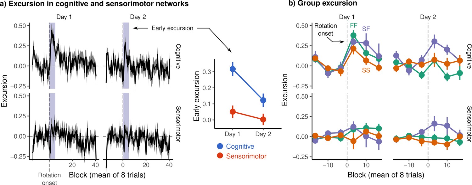
Excursion from resting manifold structure.
(a) (Left) Mean excursion in cognitive and sensorimotor networks on each day. In order to isolate the effect of rotation, subject excursion curves were standardized with respect to baseline. Vertical dashed line denotes the onset of rotation. (Right) Early excursion, defined as the mean excursion during the first 4 eight-trial blocks (shaded region in left panel), analogous to our definition of early error. (b) Mean excursion for each behavioral group. Error bars represent standard errors.
Figure 3—figure supplement 1
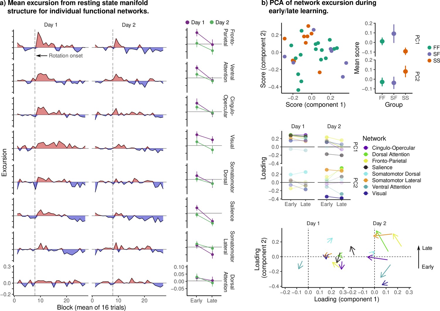
Excursion for individual Seitzman networks.
(a, Left) Excursion from resting-state manifold structure in individual networks. Networks are sorted by mean early excursion on day 1 in order to make the trends in the data more clear. Note the peak in excursion after rotation onset on day 1, most prominent in frontal and parietal cognitive networks. We also observed sustained excursion in the visual network (comprising V1 and its periphery). Although we cannot speak definitively as to its cause, it may reflect some degree of top-down modulation of the visual cortex during adaptation, so as to orient spatial attention away from the location of the stimulus, or visual feedback processing (such as the feedback related to visual errors). We also contrast the high excursion in the ventral attention network (VAN) with the near absence in the dorsal attention network (DAN). In our embedding of the cognitive network, both components predominantly encoded changes in functional connectivity between the DAN and frontoparietal networks (FPN), with the VAN loading relatively weakly. Together, these results may suggest that excursion in our cognitive network reflects excursion in the VAN and FPN individually, or in the connectivity between FPN and DAN. We note that the DAN is frequently implicated in the top-down orientation of spatial attention, and so the change in functional connectivity between DAN and FPN may reflect the learning of the visuomotor rotation. (Right) Mean excursion during early/late learning. Error bars denote standard errors. (b) For each subject, we computed the mean excursion during early/late learning for each network and day. We then performed principal component analysis in order to characterize the dominant patterns of variability in excursion across all networks. The top panels show scores on the first two components for each subject, colored by behavioral group. Note that, as in our main analysis, the FF and SF groups are highly similar. The middle panel displays the loadings for each network across days and learning epoch. The bottom panel displays the change in loading from early to late learning on each day. Note that the first component appears to encode the overall degree of excursion in each network, while the second encodes changes in excursion from early to late learning (particularly on day 2).
Figure 4
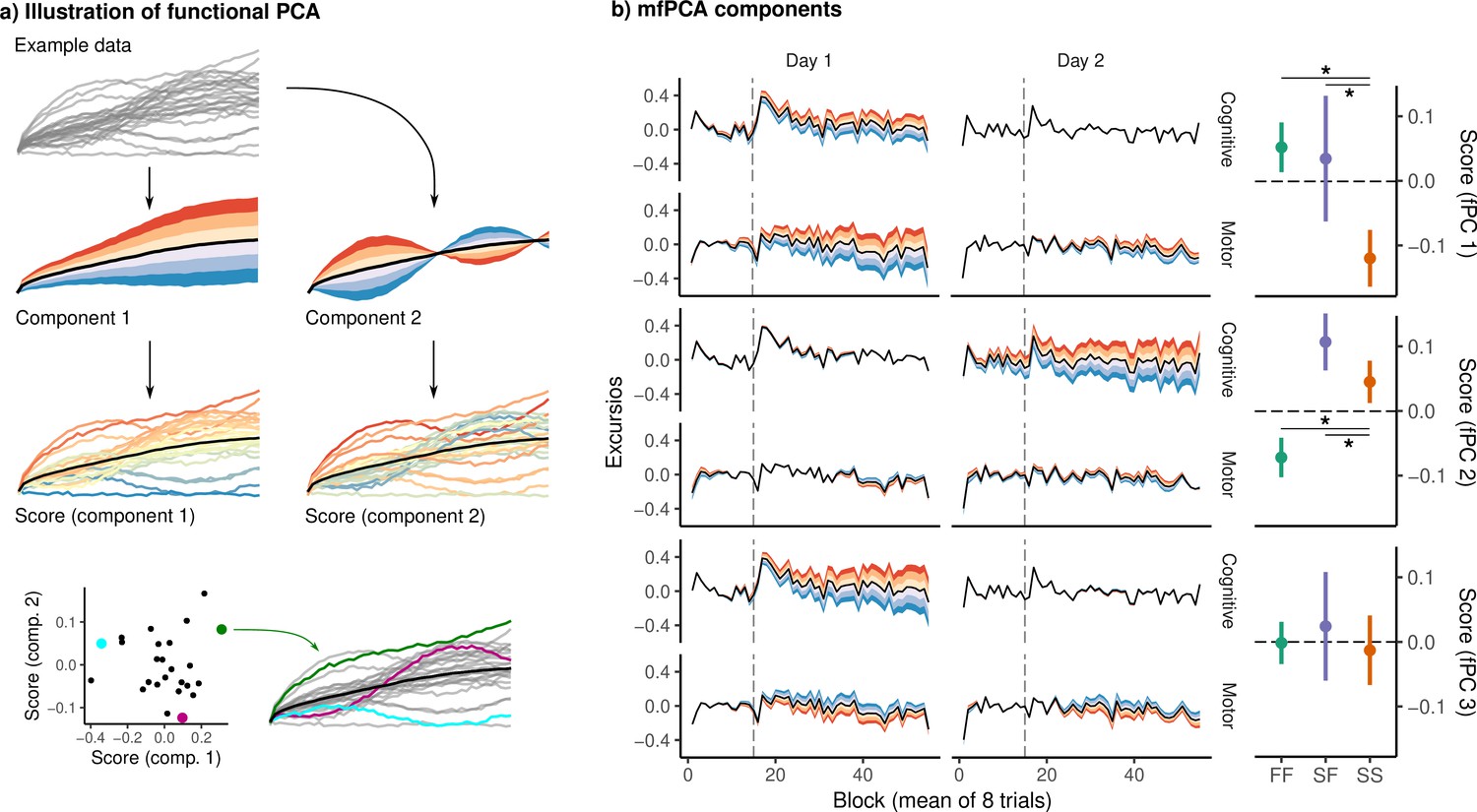
Functional principal component analysis (fPCA) of network excursion data.
(a) An example illustration of fPCA. Given a set of curves (top), fPCA extracts components describing the dominant patterns of variability in functional data (second row). In this example, the first component encodes whether the curve is higher or lower than average, while the second encodes a sinusoidal pattern in which the curve begins higher or lower than average, and then reverses direction. The score associated with a component then describes the degree to which that component is expressed in a particular observation (third row). These scores provide a low-dimensional representation of the overall shape of the curve. For example, in the bottom row, we see three example curves, and their corresponding scores on the two components. (b) Functional principal components extracted from subject excursion curves. Each panel corresponds to a single component, representing a pattern of variability in excursion across each network and day. The left panel illustrates each component as a deviation from the mean excursion (solid black line). Red (resp. blue) bands denote the effect of positive (resp. negative) scores. The right panel shows the mean score in each group. Error bars denote standard errors, while stars denote significant differences for pairwise Conover-Iman tests with Benjamini-Hochberg correction for multiple comparisons within each component.
Figure 5 with 1 supplement
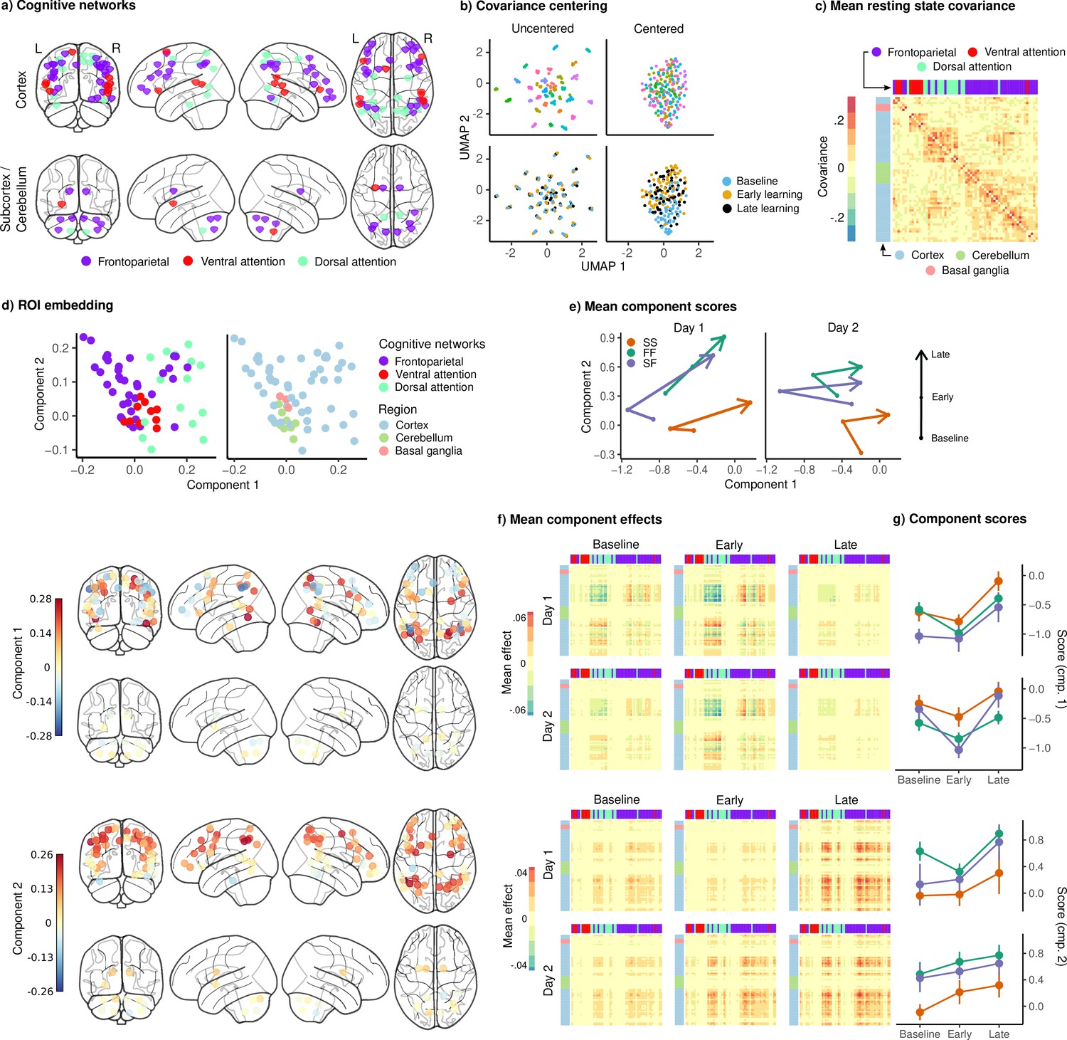
Joint embedding of cognitive networks.
(a) Regions of interest (ROIs) comprising the cognitive networks, colored by the functional network assignment of Power et al., 2011. (b) Visualization of covariance matrices by uniform manifold approximation (UMAP; McInnes et al., 2018). Each dot represents a single covariance matrix. Covariance matrices are shown both before and after centering, and are colored by subject (top) and scan (bottom). Note the strong subject-level clustering in each network before centering, which masks differences in task structure. (c) Grand mean resting-state covariance (across all subjects), to which subject task data were centered. Matrix was ordered using single-linkage hierarchical clustering. (d) (Top) Components extracted by the embedding. ROIs are colored by functional network assignment (left) and anatomical location (right). (Bottom) Embedding components displayed on the brain. ROIs are colored by their loading on each component. (e) Mean component score in each group for each task epoch and day. Arrow denotes the direction of time (baseline to early learning to late learning). (f) Components displayed as tangent vectors, reflecting changes in functional connectivity relative to rest. Each matrix represents the overall mean effect in each task epoch and day. All matrices are ordered identically to the grand mean resting-state covariance, for ease of comparison. (g) Components scores for each group during each task epoch and day. Error bars denote standard errors.
Figure 5—figure supplement 1
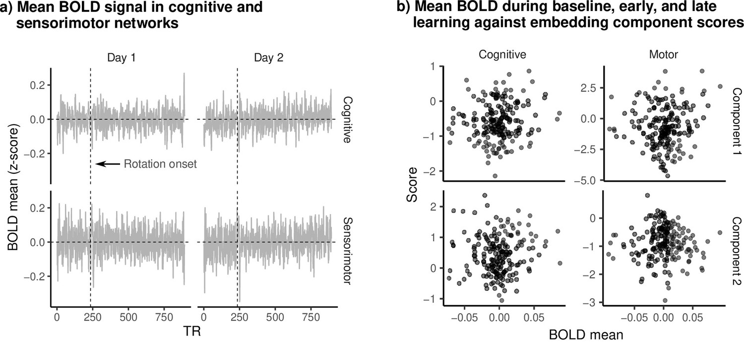
Mean BOLD signal and embedding component scores.
(a) Mean (standardized) BOLD for cognitive and sensorimotor networks during learning. Vertical dashed line denotes the onset of the visuomotor rotation. (b) Mean BOLD signal during baseline, early, and late learning epochs plotted against embedding component scores. Each dot is a single epoch (baseline, early, late learning) from a single subject. We observed no clear relationship between BOLD magnitude and scores on either component, suggesting that changes in components during learning were not simply due to widespread increase/reduction in the BOLD signal.
Figure 6
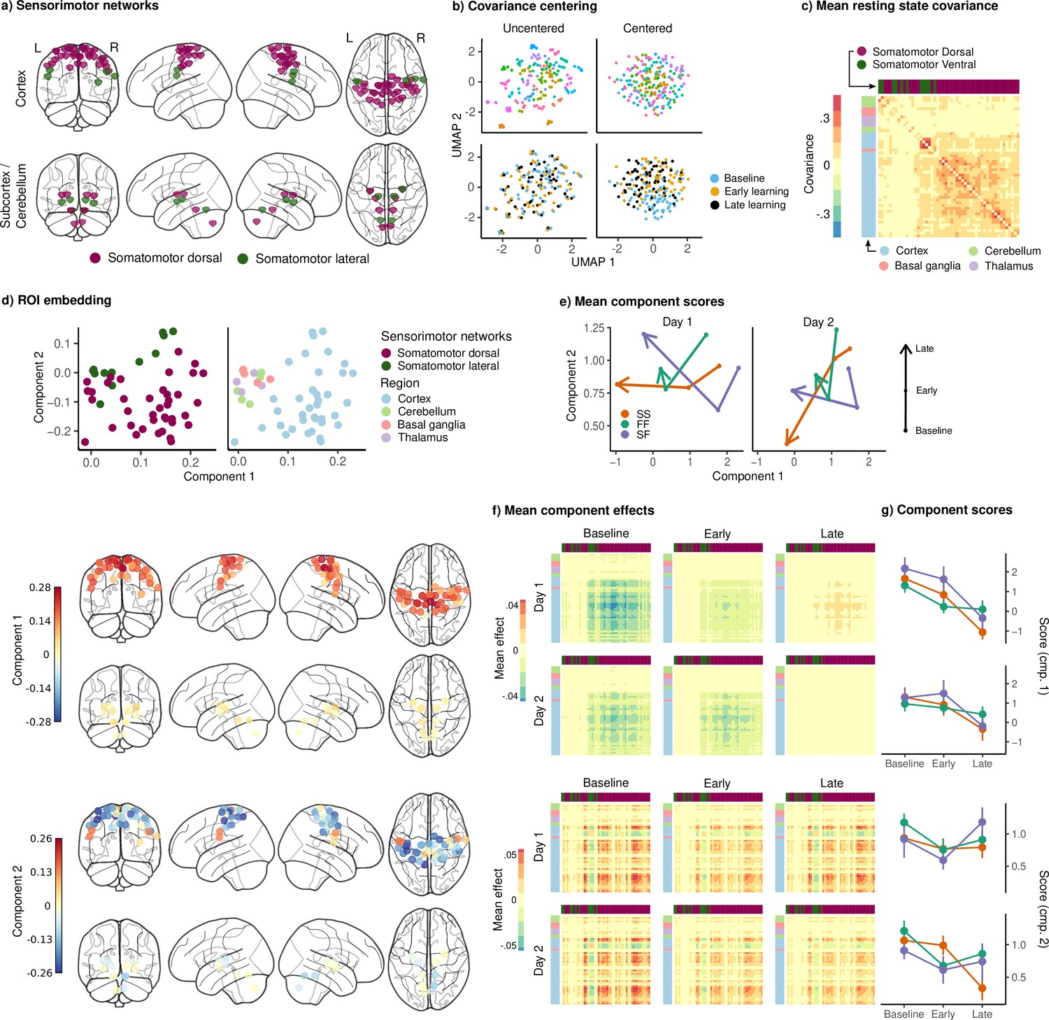
Joint embedding of sensorimotor networks.
(a) Regions of interest (ROIs) comprising the sensorimotor networks, colored by the functional network assignment of Power et al., 2011. (b) Visualization of covariance matrices by uniform manifold approximation (UMAP; McInnes et al., 2018). Each dot represents a single covariance matrix. Covariance matrices are shown both before and after centering, and are colored by subject (top) and scan (bottom). Note the strong subject-level clustering in each network before centering, which masks differences in task structure. (c) Grand mean resting-state covariance (across all subjects), to which subject task data were centered. Matrix was ordered using single-linkage hierarchical clustering. (d) (Top) Components extracted by the embedding. ROIs are colored by functional network assignment (left) and anatomical location (right). (Bottom) Embedding components displayed on the brain. ROIs are colored by their loading on each component. (e) Mean component score in each group for each task epoch and day. Arrow denotes the direction of time (baseline to early learning to late learning). (f) Components displayed as tangent vectors, reflecting changes in functional connectivity relative to rest. Each matrix represents the overall mean effect in each task epoch and day. All matrices are ordered identically to the grand mean resting-state covariance, for ease of comparison. (g) Components scores for each group during each task epoch and day. Error bars denote standard errors.
Additional files
Download links
A two-part list of links to download the article, or parts of the article, in various formats.
Downloads (link to download the article as PDF)
Open citations (links to open the citations from this article in various online reference manager services)
Cite this article (links to download the citations from this article in formats compatible with various reference manager tools)
Neural excursions from manifold structure explain patterns of learning during human sensorimotor adaptation
eLife 11:e74591.
https://doi.org/10.7554/eLife.74591


