Distance estimation from monocular cues in an ethological visuomotor task
Figures
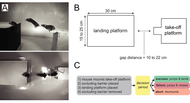
Mouse distance estimation (jumping) task.
(A) Example side and top-down video frames (three overlaid) from a single trial. (B) A random combination of landing platform width (three sizes) and gap distance (seven distances) is chosen for each trial. (C) Trial logic.
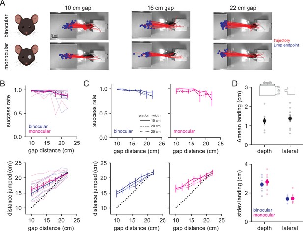
Mice accurately judge distance under binocular and monocular conditions.
(A) Example jump trajectories from a single mouse (red line is trajectory of left ear tracked by DeepLabCut, blue dot is end point of jump) at three distances for binocular (top row) and monocular (bottom row) trials. (B) Performance (top) and accuracy (bottom) in binocular (blue, n = 8 mice) and monocular (magenta, n = 8 mice) conditions averaged across landing platform widths. Thin lines are individual animal data. (C) Performance (top) and distance jumped (bottom) for bi/monocular conditions by landing platform width (indicated by line style). (D) Change in the mean landing position (top) and standard deviation of landing position (bottom) for binocular vs. monocular conditions. Smaller points are individual animal data.

Binocular vs. monocular task performance.
(A) Rates of failure (left column), success (middle column), and abort trials (right column) for binocular (blue) and monocular (magenta) conditions.
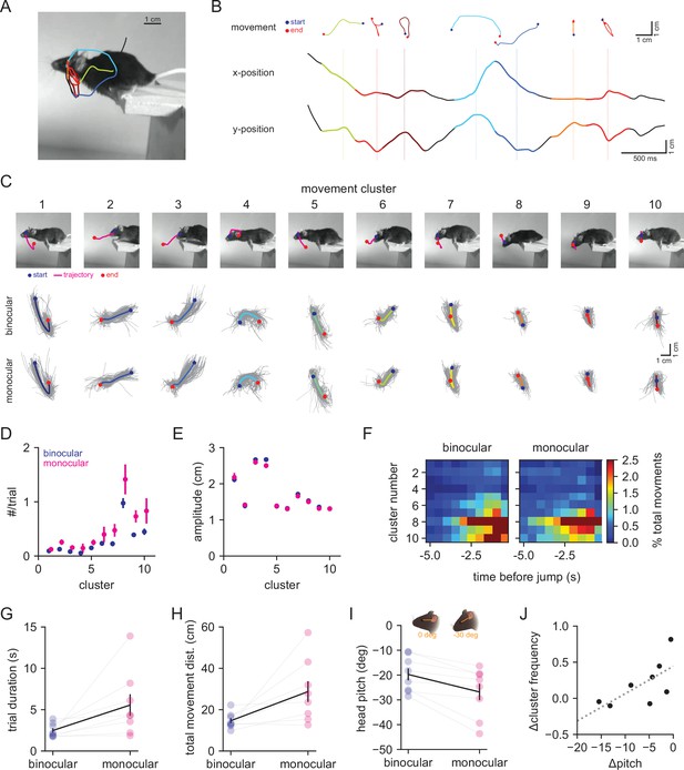
Mice perform more head movements during the decision period under monocular conditions.
(A) Example decision period trajectory of the left eye position overlaid with movements identified through velocity zero crossings. Color corresponds to movement cluster identity in (B ,C). Image is the last time point in the decision period. (B) Horizontal (x) and vertical (y) positions of eye across time from the trace in (A). Individual movements are plotted above as x/y traces, with dotted lines corresponding to the middle time point, and blue and red points indicating the start and end, respectively. Colors correspond to clusters in (C). (C) Top: example individual movements from 10 k-means clusters; magenta is the trajectory, blue and red are start and end points, respectively. Bottom: individual movement clusters for binocular (top row) and monocular (bottom row) conditions, with means plotted over 100 individual examples in gray. (D) Mean number of movements per trial for each cluster in binocular (blue) vs. monocular (magenta) conditions. (E) Mean amplitude of movement clusters for binocular (blue) and monocular (magenta) conditions. (F) Normalized movement frequency as a function of time before the jump for all clusters. (G) Mean trial duration (decision period only) for the two conditions. (H) Mean of the total distance traveled by the eye during the decision period for the two conditions. (I) Mean head pitch, measured as the angle between the eye and ear, across the decision period for the two conditions. (J) Relationship between the change in head pitch and change in cluster frequency between the binocular and monocular conditions. Dotted line is fit from linear regression.
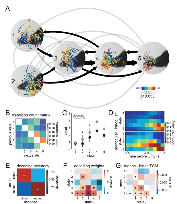
Autoregressive hidden Markov(ARHMM) modeling of decision period behavior.
(A) Example traces of eye position from five movement states labeled with autoregressive hidden Markov modeling of DeepLabCut-tracked points during the decision period (progressing blue to red in time) in average temporal order. Arrow line widths are proportional to transition probabilities between states (gray < 0.035 ≤ black). (B) Transition count matrix for binocular condition, showing the frequency of transitioning from one state (y-axis) to another state (x-axis) as a fraction of all unique state transitions; these values were used to generate the arrows in panel (A). (C) Frequency of each state for binocular (black) and monocular (gray) conditions. Asterisk indicates p<0.01, paired t-test. (D) Heat maps of start time histograms for each state normalized to the total number of trials for binocular (top) and monocular (bottom) conditions. (E) Twofold decoding analysis on transition count matrices for binocular vs. monocular conditions (performed within-animal, averaged across animals). (F) Z-scored weights used to decode binocular vs. monocular condition. (G) Difference between monocular and binocular transition count matrices; red transitions are more frequent in monocular, blue in binocular. n = 8 mice for all plots.
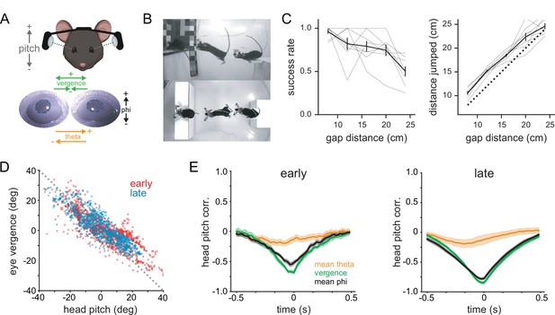
Eye movements compensate for head movements to stabilize gaze.
(A) Schematic of experimental setup for measuring head and eye movements; bilateral eye tracking with miniature head-mounted cameras (top) and ellipse fitting of DLC-tracked pupil points (bottom). (B) Side and top-view images of a mouse performing the task with the eye tracking system (three frames overlaid). (C) Performance (left) and distance jumped (right) for eye-tracking experiments. Gray lines are individual animal data. (D) Horizontal angle between the two eyes (eye theta divergence) as a function of head pitch during the decision period. ‘Early’ is from the start of the trial to 2 s before the jump, and ‘late’ is the 2 s preceding the jump. (E) Mean eye theta, eye theta vergence, and eye phi cross-correlations with head pitch angle for early (left) and late (right) portions of the decision period; n = 8 mice for all plots.
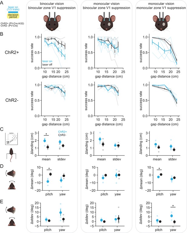
V1 optogenetic suppression disrupts distance estimation task performance.
(A) Schematic of experimental setup for optogenetic experiments; bilateral illumination of either binocular or monocular zone V1 in either binocular or monocular animals during the decision period on one-third of trials. All plots within a column correspond to the schematized condition. (B) Performance curves for laser-off (black) and laser-on (cyan) conditions in mice expressing ChR2 in PV+ inhibitory interneurons (ChR2+, top row) or PV-Cre only mice (ChR2-, bottom row). Thin lines are individual animal data. (C) Change in the mean and standard deviation of landing positions, averaged across mice. Small circles are individual animal data. (D) Change in the mean head angle for up-down (pitch) and side-to-side (yaw) head position. (E) Same as (D) but change in standard deviation of pitch and yaw.
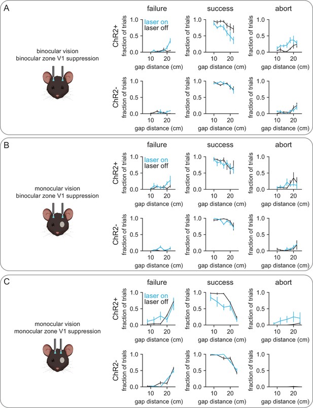
V1 optogenetic suppression task performance.
(A) Rates of failure (left column), success (middle column), and abort trials (right column) for binocular vision with optogenetic suppression of binocular zone V1. Top row shows data from animals expressing ChR2 in PV+ interneurons, and bottom row is animals lacking ChR2. Blue lines indicate laser on trials, and black lines indicate laser-off trials. (B) Same as (A) but for monocular vision with binocular zone V1 suppression. (C) Same as (B) but for monocular vision with monocular zone V1 suppression. Note that data in (C) were collected with different platform geometry and gap distances (see ‘Materials and methods’ for details).


