Spatial signatures of anesthesia-induced burst-suppression differ between primates and rodents
- Functional Imaging Laboratory, German Primate Center – Leibniz Institute for Primate Research, Germany
- Georg-August University of Göttingen, Germany
- International Max Planck Research School for Neurosciences, Germany
- A.I.V. Institute for Molecular Sciences, University of Eastern Finland, Finland
- Department of Neurology, Klinikum Rechts der Isar der Technischen Universität München, Germany
- Department of Neurology, Heidelberg University Hospital, Germany
- Department of Anesthesiology and Intensive Care Medicine, Klinikum Rechts der Isar der Technischen Universität München, Germany
- Department of Neurology, Asklepios Stadtklinik Bad Tölz, Germany
- Leibniz Science Campus Primate Cognition, Germany
Figures
Figure 1 with 1 supplement
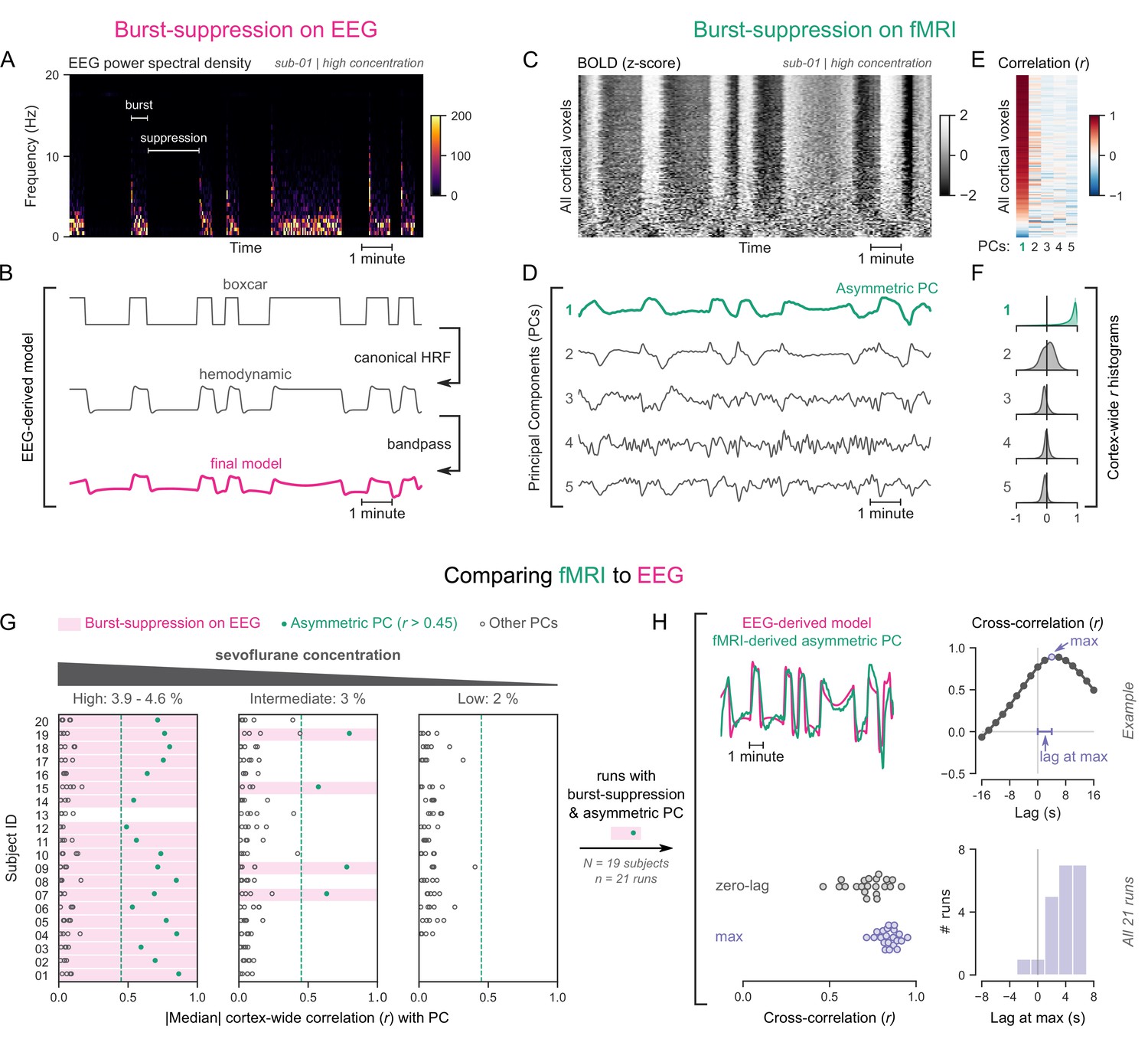
Functional magnetic resonance imaging (fMRI) signatures of electroencephalogram (EEG)-defined burst-suppression in anesthetized humans.
(A) Burst and suppression phases are marked on an EEG spectrogram of a human participant under sevoflurane anesthesia. (B) To derive the hemodynamic model of burst-suppression, the above phases (boxcar function) are convolved with a hemodynamic response function (HRF) and bandpass filtered (0.005–0.12 Hz). (C) The cortical blood-oxygen-level-dependent (BOLD) signal from the concurrent fMRI is represented as a two-dimensional matrix (carpet plot). The rows (voxels) are ordered according to their correlation with the mean cortical signal. (D) The first five temporal principal components (PCs) of the shown matrix are plotted. Cortex-wide Pearson’s correlation coefficients (r) are shown for the first PCs, both as a heatmap (E) and as histograms for each PC. (F) Taken together, panels C–F demonstrate that burst-suppression manifests as a widespread cortical BOLD signal fluctuation captured by the first PC. This component (PC1), unlike the rest, is positively correlated with most cortical voxels and is referred to as an ‘asymmetric PC’. Figure 1—figure supplement 1 shows a counterexample, that is an fMRI run acquired during the continuous slow-wave state that exhibits no asymmetric PCs. (G) To demonstrate the correspondence between burst-suppression on EEG and asymmetric PCs on fMRI across the entire human dataset, median cortex-wide r values of the first five PCs are plotted as dots for each run. The runs that exhibit burst-suppression on EEG also have a single prominent asymmetric PC with median cortex-wide r>0.45 (except for subject 15 at high concentration). (H) For these runs, the cross-correlation between EEG-derived hemodynamic models and asymmetric PCs is shown. The cross-correlation at zero-lag, the maximum cross-correlation, and the time-lag at the maximum are extracted for each run (see example in top row) and plotted across all runs (bottom row). Numerical data for panels G and H are provided in Figure 1—source data 1.
-
Figure 1—source data 1
Numerical data for Figure 1G–H.
- https://cdn.elifesciences.org/articles/74813/elife-74813-fig1-data1-v1.xlsx
Figure 1—figure supplement 1
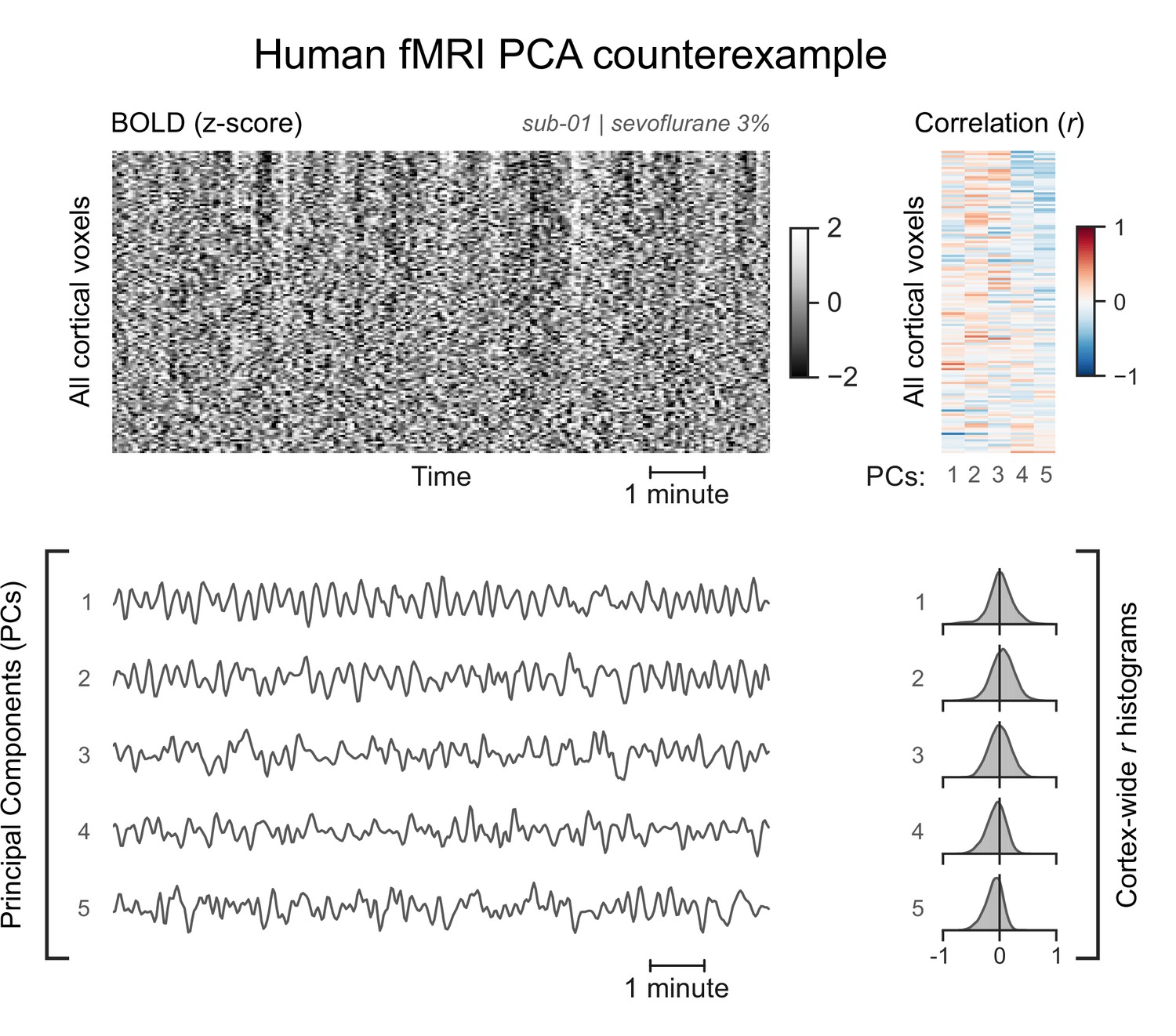
A functional magnetic resonance imaging (fMRI) run without asymmetric principal components (PCs).
The cortical blood-oxygen-level-dependent (BOLD) fMRI signal of the same human participant anesthetized with a lower concentration of sevoflurane is represented as a carpet plot. The first five temporal PCs of the signal are plotted below the carpet plot. The Pearson’s correlation coefficients (r) between the PCs and all cortical voxels are represented both as a heatmap and as histograms for each PC. All PCs have symmetric histograms, centered around r=0.
Figure 2 with 4 supplements
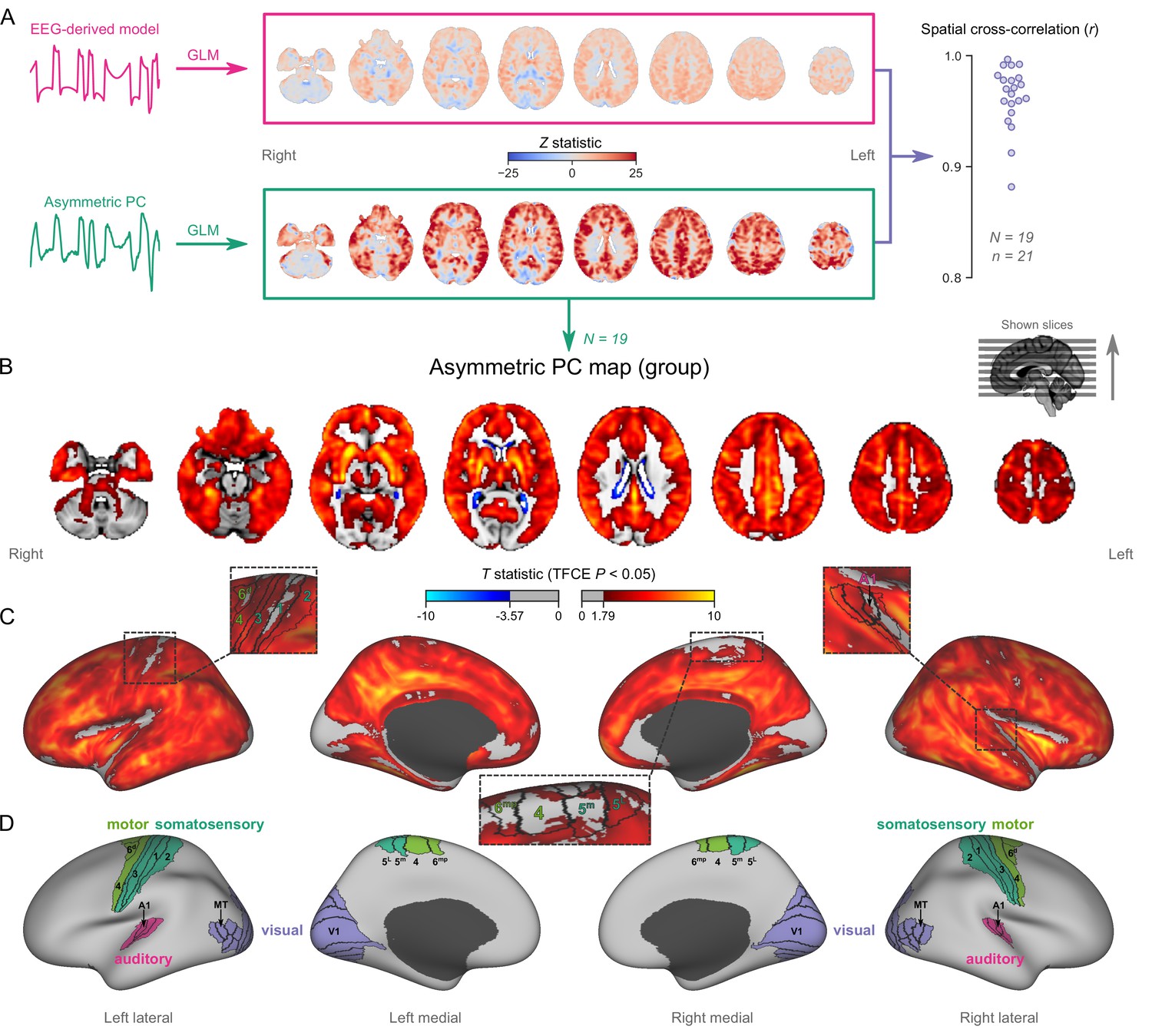
Mapping burst-suppression in anesthetized humans without electroencephalogram (EEG).
(A) Maps of burst-suppression are computed via general linear model (GLM) analysis using one of two regressors—either the EEG-derived hemodynamic model or the functional magnetic resonance imaging (fMRI)-derived asymmetric principal component (PC). The resulting Z statistic maps, for an example subject are shown here in the MNI152 template space. Neighborhood cross-correlation values between the two types of Z statistic maps are plotted on the right, across all runs with asymmetric PCs (N=19 subjects, n=21 EEG-fMRI runs, see Figure 2—source data 1). (B) The group burst-suppression map, computed via a second-level analysis of the single-subject asymmetric PC GLMs, is shown here overlaid on the MNI152 volumetric template. The group statistics were carried out with the FSL (FMRIB's Software Library) tool randomise; the resulting T statistic maps were thresholded using threshold-free cluster enhancement (TFCE) and a corrected p<0.05. Figure 2—figure supplement 1 provides a closer look at subcortical structures, while Figure 2—figure supplement 2 examines the source of the observed anticorrelation at the ventricular borders. (C) The group burst-suppression map is shown in fsaverage surface space. Non-cortical areas on the medial surface are shown in dark gray. (D) The locations of several sensory and motor cortical areas, based on the Human Connectome Project multimodal parcellation, are indicated on the surface: primary motor (area 4), premotor (areas 6d and 6mp), primary somatosensory (areas 3a–b, 1, and 2), higher somatosensory (areas 5 m and 5 L), primary auditory, higher auditory (medial and lateral belt, parabelt), primary visual, and higher-order visual (V2, V3, V3A, V3B, V4, V4t, V6, V6A, V7, V8, MT, MST, and lateral occipital areas 1–3). Figure 2—figure supplement 3 shows the unthresholded group burst-suppression map in both volumetric and surface representations. Figure 2—figure supplement 4 shows a temporal signal-to-noise ratio map overlaid on the volumetric template.
-
Figure 2—source data 1
Spatial cross-correlation values for Figure 2A.
- https://cdn.elifesciences.org/articles/74813/elife-74813-fig2-data1-v1.xlsx
Figure 2—figure supplement 1
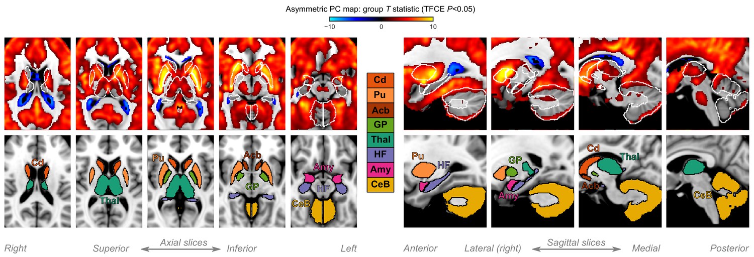
A closer look at subcortical structures.
Group statistic map showing the spatial distribution of asymmetric principal components (PCs) in humans—same as in Figure 2B. The views are adjusted to focus on subcortical structures, on axial and sagittal slices. The bottom row shows the location of major subcortical structures defined based on the human Harvard-Oxford subcortical structural atlas. Cd: caudate; Pu: putamen; Acb: accumbens; GP: globus pallidus; Thal: thalamus; HF: hippocampal formation; Amy: amygdala; CeB: cerebellum.
Figure 2—figure supplement 2
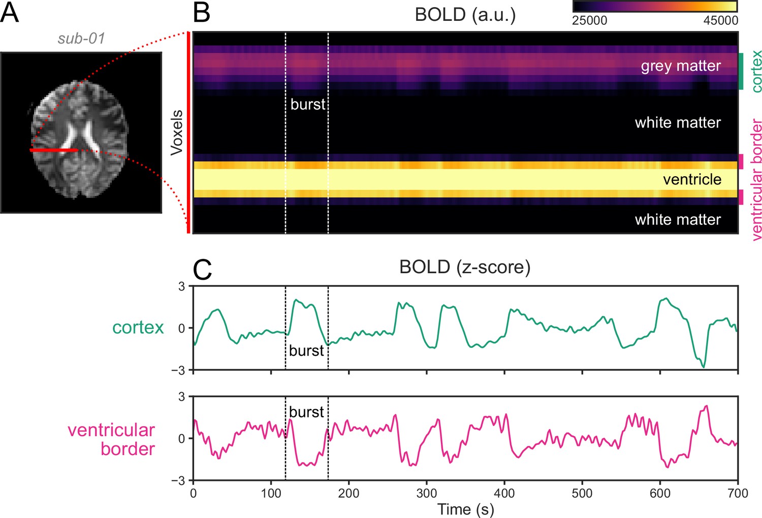
Ventricular motion during burst-suppression.
(A) An axial slice from an echo planar imaging blood-oxygen-level-dependent (BOLD) functional magnetic resonance imaging (fMRI) scan of a human subject during burst-suppression (same run as in Figure 1). A line profile is marked in red, stretching from the pial surface of the right hemisphere toward the midline, going through cortical gray matter, white matter, and the lateral ventricle. (B) The BOLD signal across this line profile is plotted for the entire duration of the fMRI run (700 s). One of the bursts is marked by vertical dashed lines. (C) During bursts, the mean BOLD signal of the cortical voxels rises—as expected, whereas the signal at the ventricular borders falls. This is most likely caused by an inward motion of the ventricular borders, with the low-intensity BOLD signal of the surrounding white matter replacing the higher-intensity ventricular signal. Even if the motion occurs on a sub-voxel scale, partial volume effects would still cause the darkening of the border.
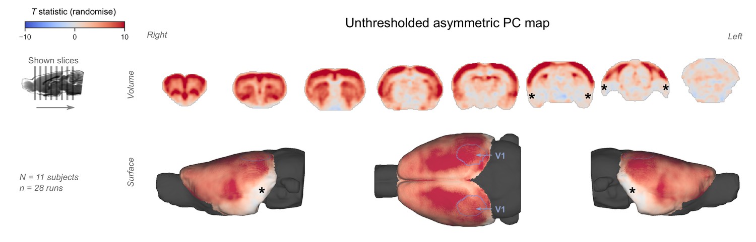
Figure 2—figure supplement 3
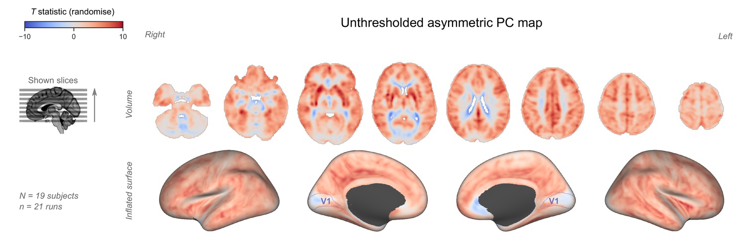
Unthresholded asymmetric principal component (PC) map.
The unthresholded group-level T statistic map is overlaid on volumetric slices and surfaces identical to the ones in Figure 2B–C. The primary visual cortex (V1) is outlined in purple.
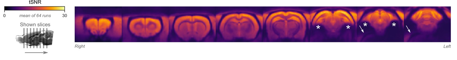
Figure 2—figure supplement 4
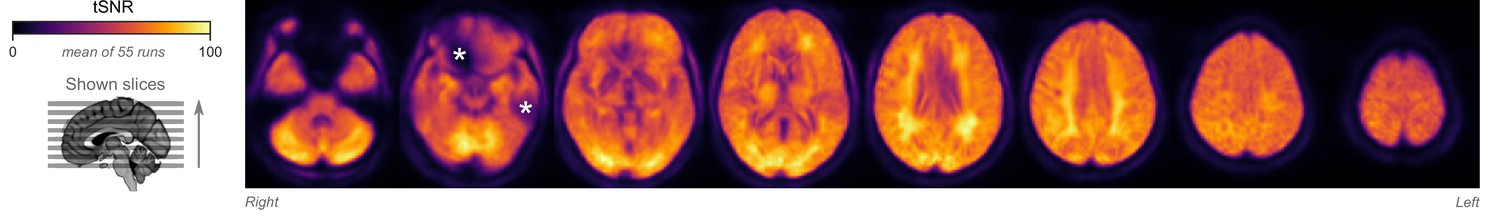
Temporal signal-to-noise ratio (tSNR) map.
The map is overlaid on volumetric slices identical to the ones in Figure 2B. For each functional magnetic resonance imaging (fMRI) run, tSNR was computed prior to preprocessing by dividing the mean of the fMRI image across time with its SD across time. The map shown here represents the average tSNR values across all analyzed fMRI runs (with or without burst-suppression). Asterisks indicate areas with low tSNR due to susceptibility-induced distortions and signal drop-outs.
Figure 3 with 4 supplements
Macaques exhibit human homologous functional magnetic resonance imaging (fMRI) signatures of burst-suppression.
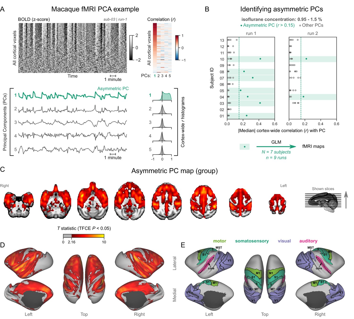
(A) The cortical blood-oxygen-level-dependent (BOLD) fMRI signal of a long-tailed macaque during isoflurane anesthesia is represented as a carpet plot. The rows (voxels) are ordered according to their correlation with the mean cortical signal. The first five temporal principal components (PCs) of the signal are plotted below. The Pearson’s correlation coefficients (r) between the PCs and all cortical voxels are represented both as a heatmap and as histograms for each PC. The first PC captures the widespread fluctuation visible on the carpet plot and has an asymmetric r histogram. Figure 3—figure supplement 1 shows a counterexample, that is an fMRI run that exhibits no asymmetric PCs. (B) Cortex-wide median r values for the first five PCs are plotted as dots across the entire macaque dataset (see Figure 3—source data 1). The fMRI runs with a single prominent asymmetric PC (r>0.15, highlighted in green) are selected for general linear model (GLM) analysis. (C) The group asymmetric PC map, computed via a second-level analysis of single-subject GLMs, is shown here overlaid on a study-specific volumetric template. The group statistics were carried out with FSL randomise; the resulting T statistic maps were thresholded using threshold-free cluster enhancement (TFCE) and a corrected p<0.05. Figure 3—figure supplement 2 provides a closer look at subcortical structures. (D) The same group map is shown on a cortical surface representation of the template. Non-cortical areas on the medial surface are shown in dark gray. (E) The locations of several sensory and motor cortical areas, based on the cortical hierarchical atlas of the rhesus macaque, are indicated on the surface: primary visual (V1), higher-order visual (V2, V3, V4, V6, MT, MST, and FST), primary somatosensory (S1), higher somatosensory (area 5), primary motor (M1), and auditory cortices (auditory core, belt, and parabelt). Figure 3—figure supplement 3 shows the unthresholded group asymmetric PC map in both volumetric and surface representations. Figure 3—figure supplement 4 shows a temporal signal-to-noise ratio map overlaid on the volumetric template.
-
Figure 3—source data 1
Numerical data for Figure 3B.
- https://cdn.elifesciences.org/articles/74813/elife-74813-fig3-data1-v1.xlsx
Figure 3—figure supplement 1
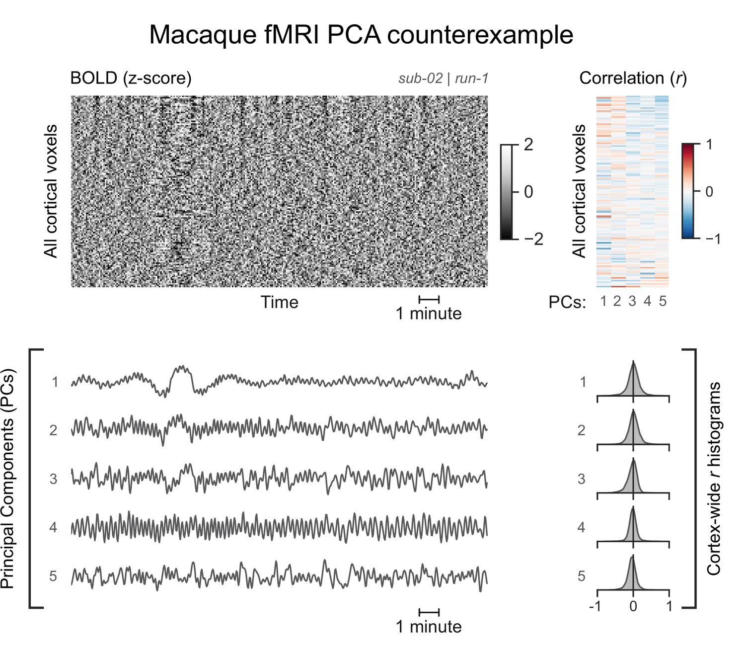
A functional magnetic resonance imaging (fMRI) run without asymmetric principal components (PCs).
The cortical blood-oxygen-level-dependent (BOLD) fMRI signal of another macaque subject is represented as a carpet plot. The first five temporal PCs of the signal are plotted below the carpet plot. The Pearson’s correlation coefficients (r) between the PCs and all cortical voxels are represented both as a heatmap and as histograms for each PC. All PCs have symmetric histograms, centered around r=0.
Figure 3—figure supplement 2
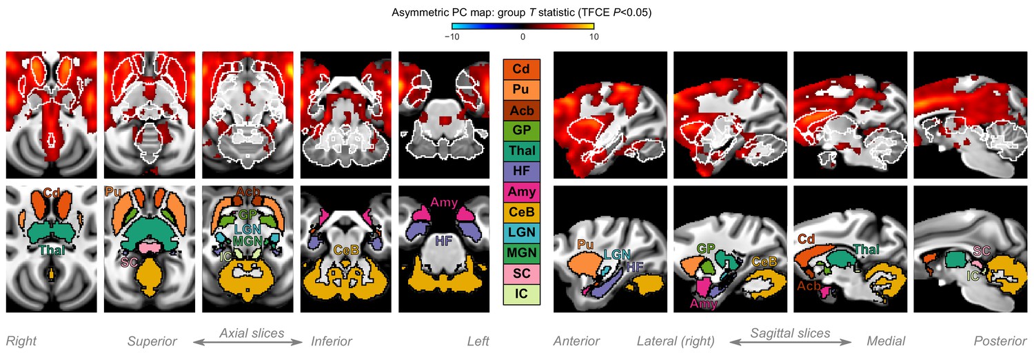
A closer look at subcortical structures.
Group statistic map showing the spatial distribution of asymmetric principal components (PCs) in macaques—same as in Figure 3C. The views are adjusted to focus on subcortical structures, on axial and sagittal slices. The bottom row shows the location of major subcortical structures defined based on the subcortical atlas of the rhesus macaque. Cd: caudate; Pu: putamen; Acb: accumbens; GP: globus pallidus; Thal: thalamus; HF: hippocampal formation; Amy: amygdala; CeB: cerebellum; LGN: lateral geniculate nucleus; MGN: medial geniculate nucleus; SC: superior colliculus; IC: inferior colliculus.
Figure 3—figure supplement 3
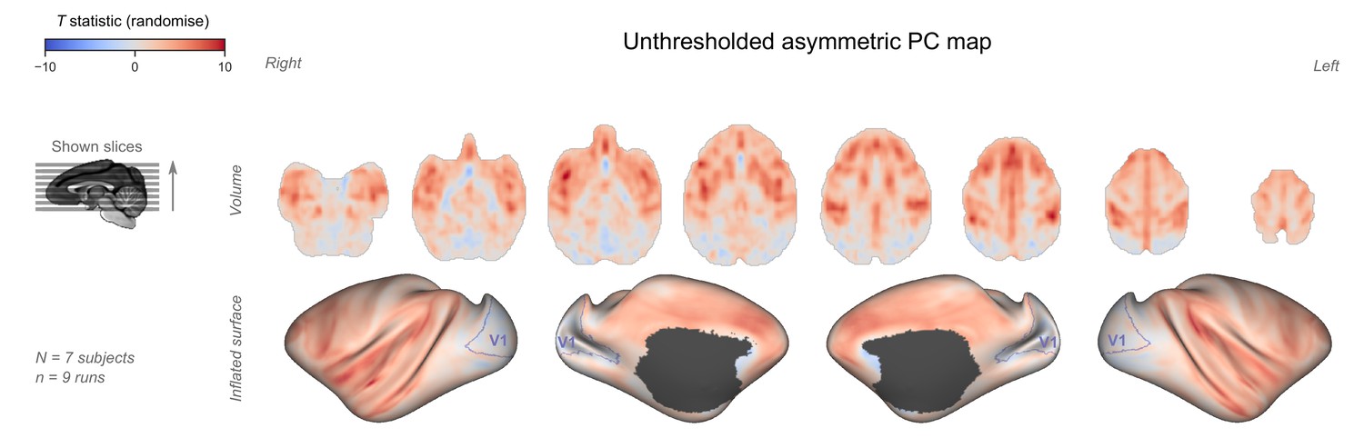
Unthresholded asymmetric principal component (PC) map.
The unthresholded group-level T statistic map is overlaid on volumetric slices and surfaces identical to the ones in Figure 3C–D. The primary visual cortex (V1) is outlined in purple.
Figure 3—figure supplement 4
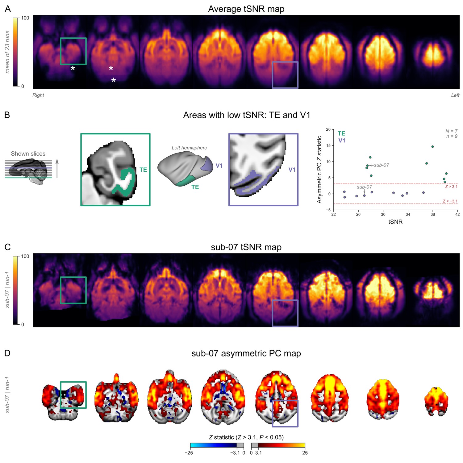
Temporal signal-to-noise ratio (tSNR) map.
(A) The map is overlaid on volumetric slices identical to the ones in Figure 3C. For each functional magnetic resonance imaging (fMRI) run, tSNR was computed prior to preprocessing by dividing the mean of the fMRI image across time with its SD across time. The map shown here represents the average tSNR values across all analyzed fMRI runs (with or without burst-suppression). Asterisks indicate areas with low tSNR, either due to increased distance from the coil (cerebellum) or due to susceptibility-induced distortions and signal drop-outs (areas close to the ear canals). (B) The locations of two areas with low tSNR values—primary visual cortex (V1) and area TE of the inferior temporal cortex—are shown on the left hemisphere. The two areas have comparable tSNR values but differ in their correlation to the asymmetric principal component (PC) (see Figure 3—figure supplement 4—source data 1). Dashed lines indicate the cluster-defining Z statistic thresholds applied during the first-level general linear model (GLM) analysis. (C) The tSNR map for an example fMRI run (sub-07, run-1). (D) The asymmetric PC map (output of first-level GLM) for the same run.
-
Figure 3—figure supplement 4—source data 1
Numerical data for Figure 3—figure supplement 4B.
- https://cdn.elifesciences.org/articles/74813/elife-74813-fig3-figsupp4-data1-v1.xlsx
Figure 4 with 5 supplements
Marmosets exhibit human homologous functional magnetic resonance imaging (fMRI) signatures of burst-suppression.
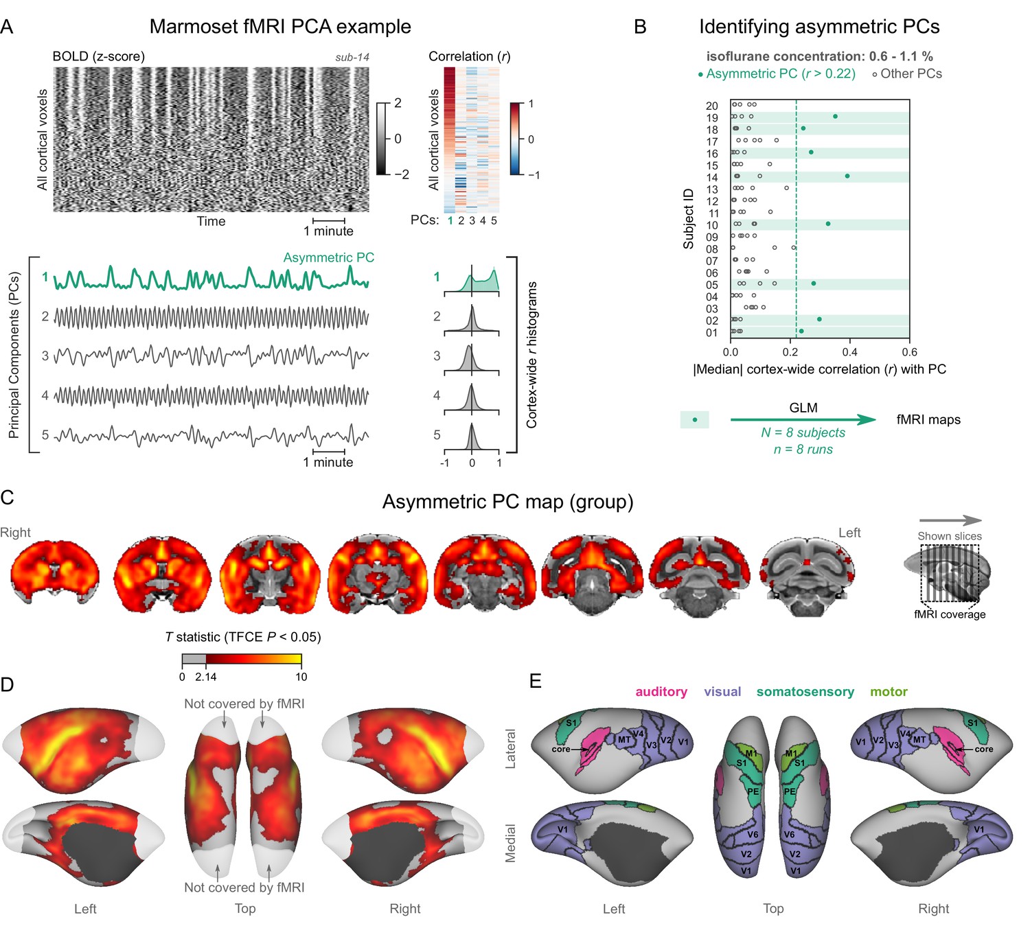
(A) The cortical blood-oxygen-level-dependent (BOLD) fMRI signal of a common marmoset during isoflurane anesthesia is represented as a carpet plot, with rows (voxels) ordered according to their correlation with the mean cortical signal. The first five temporal principal components (PCs) of the signal are plotted below. The Pearson’s correlation coefficients (r) between the PCs and all cortical voxels are represented both as a heatmap and as histograms for each PC. The first PC captures the widespread fluctuation visible on the carpet plot and has an asymmetric r histogram. Figure 4—figure supplement 1 shows a counterexample, an fMRI run that exhibits no asymmetric PCs. (B) Cortex-wide median r values for the first five PCs are plotted as dots across the entire marmoset dataset (see Figure 4—source data 1). The fMRI runs with a single prominent asymmetric PC (r>0.22, highlighted in green) are selected for general linear model (GLM) analysis. (C) The group asymmetric PC map, computed via a second-level analysis of single-subject GLMs, is shown here overlaid on the NIH v3.0 population template (T2-weighted image). The group statistics were carried out with FSL randomise; the resulting T statistic maps were thresholded using threshold-free cluster enhancement (TFCE) and a corrected p<0.05. Figure 4—figure supplement 2 provides a closer look at subcortical structures. (D) The same group map is shown on a cortical surface representation of the template. Non-cortical areas on the medial surface are shown in dark gray. Areas not covered by the fMRI volume are shown in white. (E) The locations of several sensory and motor cortical areas, according to the NIH MRI-based cortical parcellation, are indicated on the surface: primary visual (V1), higher-order visual (V2, V3, V4, V6, MT, MST, and Brodmann area 19), primary somatosensory (S1), higher somatosensory (area PE), primary motor (M1), and auditory cortices (auditory core, belt, parabelt, and superior temporal rostral area). Figure 4—figure supplement 3 shows the unthresholded group asymmetric PC map in both volumetric and surface representations. Figure 4—figure supplement 4 shows a temporal signal-to-noise ratio map overlaid on the volumetric template. Figure 4—figure supplement 5 shows results from an additional marmoset in which the whole brain was covered by the fMRI volume.
-
Figure 4—source data 1
Numerical data for Figure 4B.
- https://cdn.elifesciences.org/articles/74813/elife-74813-fig4-data1-v1.xlsx
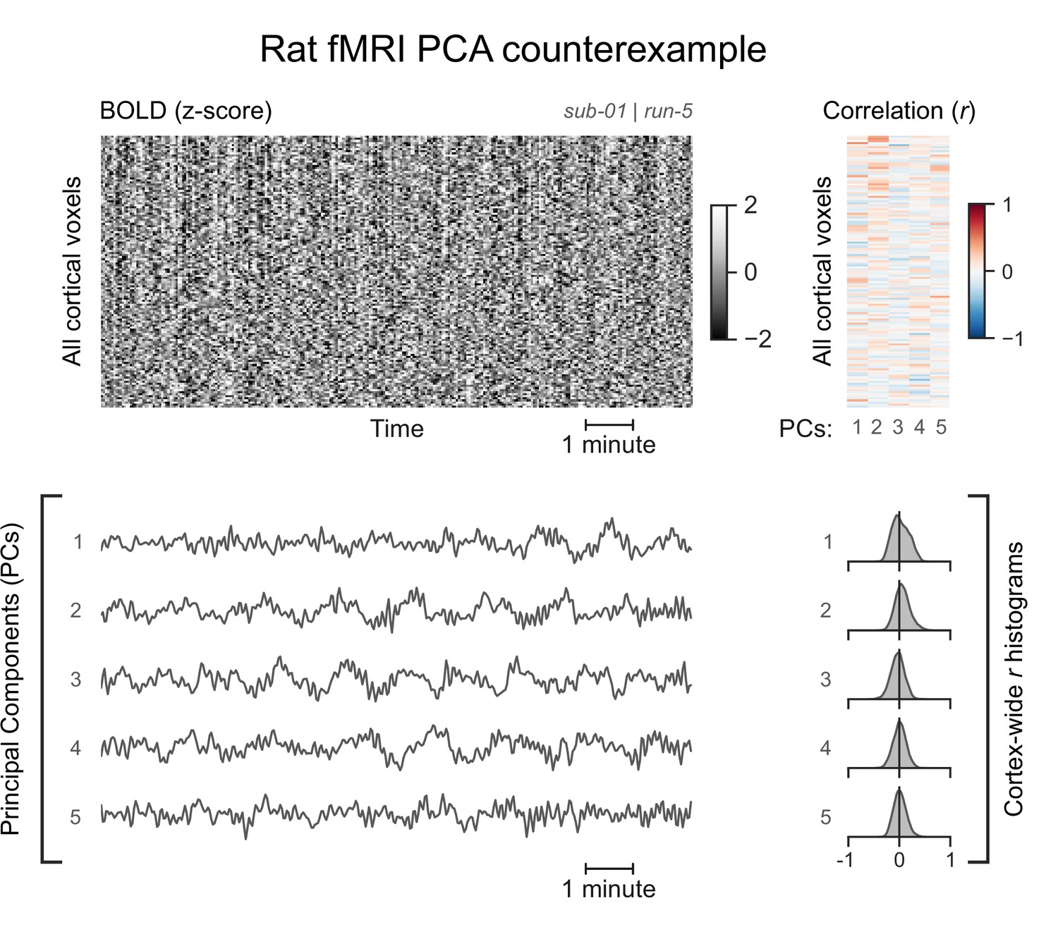
Figure 4—figure supplement 1
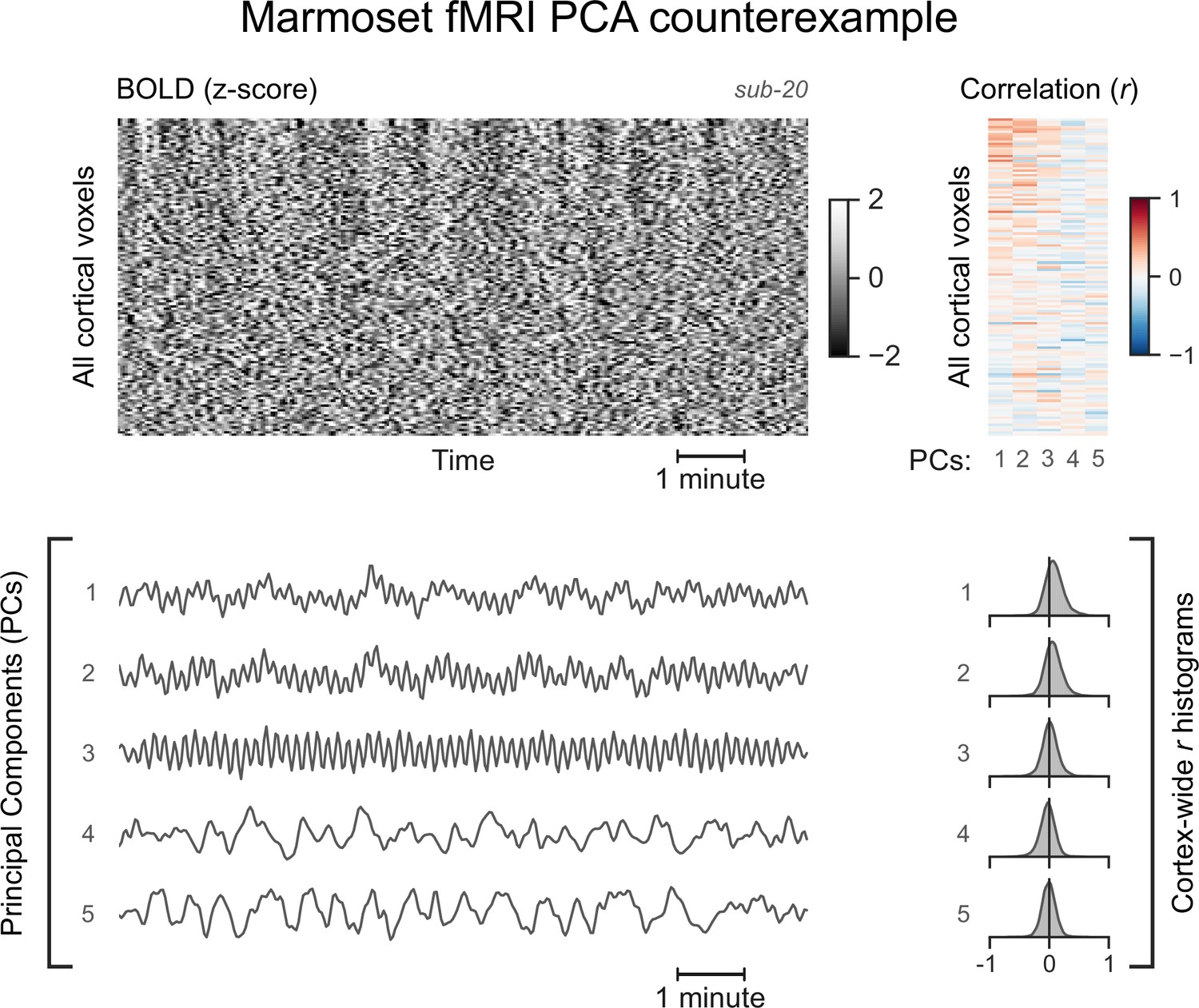
A functional magnetic resonance imaging (fMRI) run without asymmetric principal components (PCs).
The cortical blood-oxygen-level-dependent (BOLD) fMRI signal of another marmoset subject is represented as a carpet plot. The first five temporal PCs of the signal are plotted below the carpet plot. The Pearson’s correlation coefficients (r) between the PCs and all cortical voxels are represented both as a heatmap and as histograms for each PC. All PCs have symmetric histograms, centered around r=0.
Figure 4—figure supplement 2
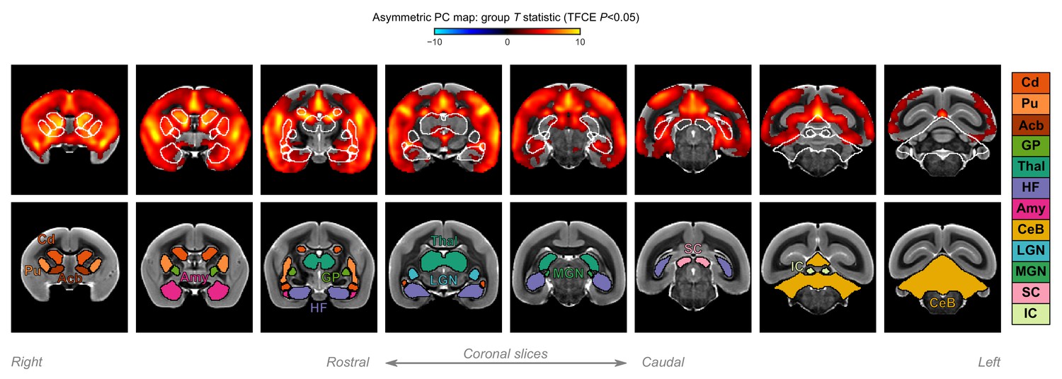
A closer look at subcortical structures.
Group statistic map showing the spatial distribution of asymmetric principal components (PCs) in marmosets—same as in Figure 4C. The views are adjusted to focus on subcortical structures. The bottom row shows the location of major subcortical structures defined based on the marmoset brain mapping coarse subcortical atlas. Cd: caudate; Pu: putamen; Acb: accumbens; GP: globus pallidus; Thal: thalamus; HF: hippocampal formation; Amy: amygdala; CeB: cerebellum; LGN: lateral geniculate nucleus; MGN: medial geniculate nucleus; SC: superior colliculus; IC: inferior colliculus.
Figure 4—figure supplement 3
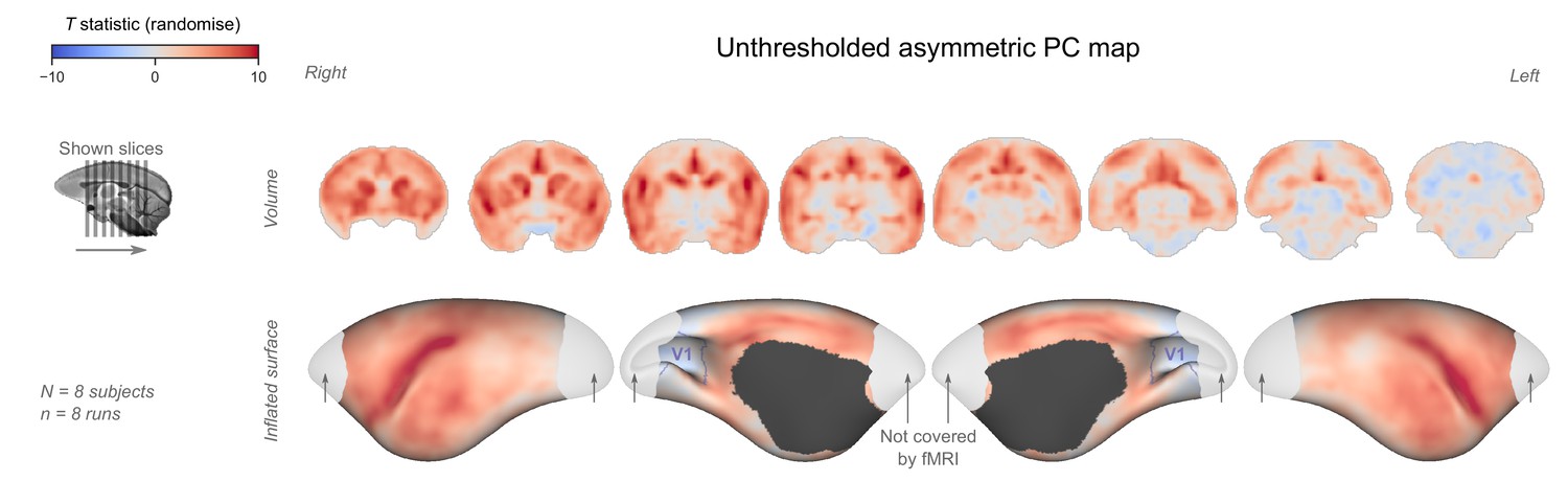
Unthresholded asymmetric principal component (PC) map.
The unthresholded group-level T statistic map is overlaid on volumetric slices and surfaces identical to the ones in Figure 4C–D. The primary visual cortex (V1) is outlined in purple.
Figure 4—figure supplement 4
Temporal signal-to-noise ratio (tSNR) map.
The map is overlaid on volumetric slices identical to the ones in Figure 4C. For each fMRI run, tSNR was computed prior to preprocessing by dividing the mean of the fMRI image across time with its SD across time. The map shown here represents the average tSNR values across all analyzed fMRI runs (with or without burst-suppression). Asterisks indicate areas with low tSNR, either due to increased distance from the coil or due to susceptibility-induced distortions and signal drop-outs.
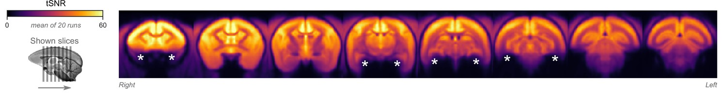
Figure 4—figure supplement 5
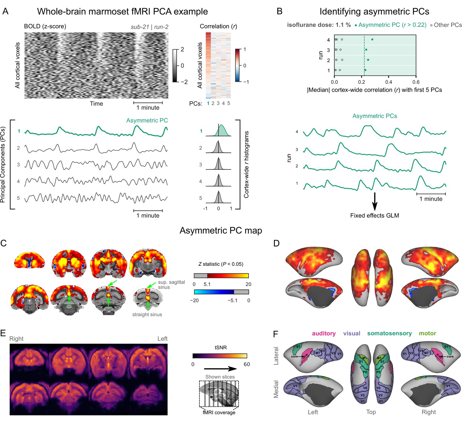
Marmoset burst-suppression map with whole-brain coverage.
The data shown here come from an additional marmoset (sub-21) in which the whole brain was imaged. (A) An example of an asymmetric principal component (PC) is depicted in the same way as in Figure 4A. (B) Asymmetric PCs (median cortex-wide r>0.22) were found in all four fMRI runs acquired in this marmoset (see Figure 4—figure supplement 5—source data 1) and were selected for GLM analysis. (C) The asymmetric PC map, computed via a fixed-effects analysis of the four fMRI runs, is shown here overlaid on the NIH v3.0 population template (T2-weighted image). The Z statistic image was thresholded non-parametrically using gaussian random field theory-based maximum height thresholding with a (corrected) significance threshold of p=0.05. Green arrows indicate the locations of the superior sagittal and straight sinuses which exhibit significant correlation with the asymmetric PCs. (D) The same map is shown on a cortical surface representation of the template. (E) A temporal signal-to-noise ratio map (tSNR, average across the four runs) is shown overlaid on the volumetric template. (F) The locations of several sensory and motor cortical areas (the same as in Figure 4E) are indicated on the surface.
-
Figure 4—figure supplement 5—source data 1
Numerical data for Figure 4—figure supplement 5B.
- https://cdn.elifesciences.org/articles/74813/elife-74813-fig4-figsupp5-data1-v1.xlsx
Figure 5 with 5 supplements

Rats exhibit pancortical functional magnetic resonance imaging (fMRI) signatures of burst-suppression.
(A) The cortical blood-oxygen-level-dependent (BOLD) fMRI signal of a rat during isoflurane (2%) anesthesia is represented as a carpet plot, with rows (voxels) ordered according to their correlation with the mean cortical signal. The first five temporal principal components (PCs) of the signal are plotted below. The Pearson’s correlation coefficients (r) between the PCs and all cortical voxels are represented both as a heatmap and as histograms for each PC. The first PC captures the widespread fluctuation visible on the carpet plot and has an asymmetric r histogram. Figure 5—figure supplement 1 shows a counterexample, an fMRI run that exhibits no asymmetric PCs. (B) Cortex-wide median r values for the first five PCs are plotted as dots across the entire rat dataset (see Figure 5—source data 1). fMRI runs with a single prominent asymmetric PC (r>0.2, highlighted in green) are selected, excluding runs that had a second PC within r=0.15 of the most asymmetric PC (marked with an asterisk). The selected 28 runs serve as inputs for general linear model (GLM) analysis. (C) The group asymmetric PC map, computed via a second-level analysis of single-subject GLMs, is shown here overlaid on a study-specific volumetric template. The group statistics were carried out with FSL randomise; the resulting T statistic maps were thresholded using threshold-free cluster enhancement (TFCE) and a corrected p<0.05. Figure 5—figure supplement 2 provides a closer look at subcortical structures. (D) The same group map is shown on a cortical surface representation of the template. The cerebellum and the olfactory bulb are shown in dark gray. (E) The locations of primary motor, somatosensory, auditory, and visual cortices—based on the SIGMA rat brain atlas—are indicated on the surface. Figure 5—figure supplement 3 shows the unthresholded group asymmetric PC map in both volumetric and surface representations. Figure 5—figure supplement 4 shows a temporal signal-to-noise ratio map overlaid on the volumetric template. In Figure 5—figure supplement 5, the asymmetric PC map is reproduced in a second rat fMRI dataset (Rat 2) from a previously published study.
-
Figure 5—source data 1
Numerical data for Figure 5B.
- https://cdn.elifesciences.org/articles/74813/elife-74813-fig5-data1-v1.xlsx
Figure 5—figure supplement 1
A functional magnetic resonance imaging (fMRI) run without asymmetric principal components (PCs).
The cortical blood-oxygen-level-dependent (BOLD) fMRI signal of the same rat subject anesthetized with a lower concentration of isoflurane (1.5%) is represented as a carpet plot. The first five temporal PCs of the signal are plotted below the carpet plot. The Pearson’s correlation coefficients (r) between the PCs and all cortical voxels are represented both as a heatmap and as histograms for each PC. All PCs have symmetric histograms, centered around r=0.
Figure 5—figure supplement 2
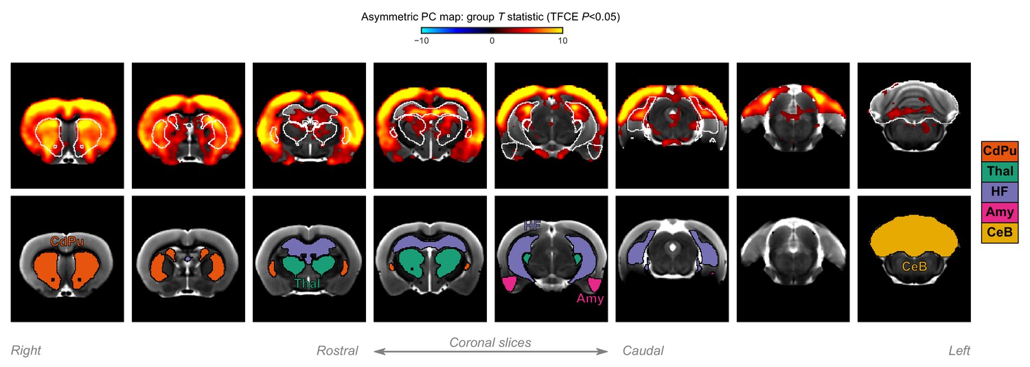
A closer look at subcortical structures.
Group statistic map showing the spatial distribution of asymmetric principal components (PCs) in rats—same as in Figure 5C. The views are adjusted to focus on subcortical structures. The bottom row shows the location of major subcortical structures, defined based on the SIGMA rat brain atlas. CdPu: caudate-putamen; Thal: thalamus; HF: hippocampal formation; Amy: amygdala; CeB: cerebellum.
Figure 5—figure supplement 3
Unthresholded asymmetric principal component (PC) map.
The unthresholded group-level T statistic map is overlaid on volumetric slices and surfaces identical to the ones in Figure 5C–D. The primary visual cortex (V1) is outlined in purple. Asterisks indicate areas with low signal-to-noise ratio (see also Figure 4).
Figure 5—figure supplement 4
Temporal signal-to-noise ratio (tSNR) map.
The map is overlaid on volumetric slices identical to the ones in Figure 5C. For each functional magnetic resonance imaging (fMRI) run, tSNR was computed prior to preprocessing by dividing the mean of the fMRI image across time with its SD across time. The map shown here represents the average tSNR values across all analyzed fMRI runs (with or without burst-suppression). Asterisks indicate areas with low tSNR due to susceptibility-induced distortions and signal drop-outs. Arrows indicate an EPI ghost artifact.
Figure 5—figure supplement 5
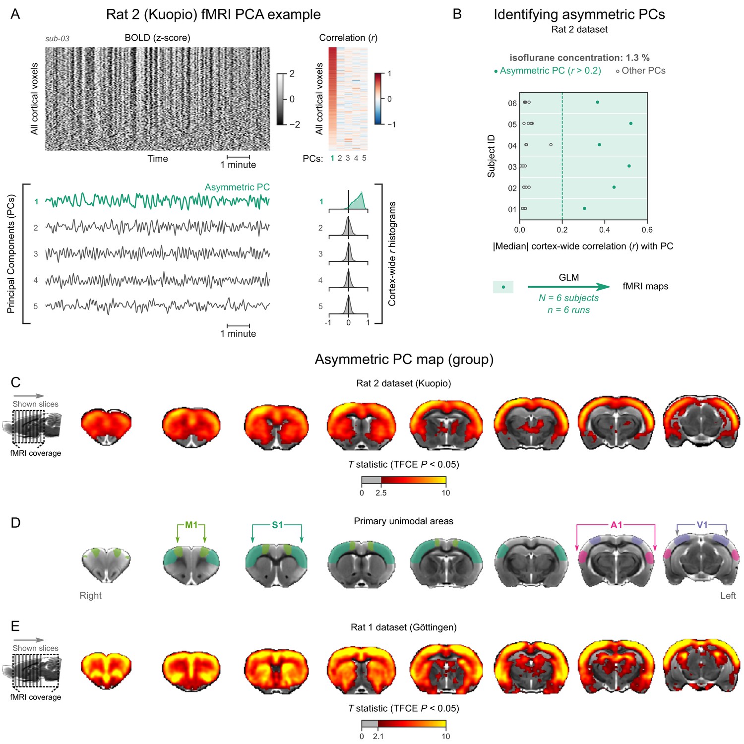
Identifying and mapping asymmetric principal components (PCs) in the Rat 2 dataset.
(A) The cortical blood-oxygen-level-dependent (BOLD) functional magnetic resonance imaging (fMRI) signal of an isoflurane-anesthetized subject from the Rat 2 dataset is represented as a carpet plot. The first five temporal PCs of the signal are plotted below the carpet plot. The Pearson’s correlation coefficients (r) between the PCs and all cortical voxels are represented both as a heatmap and as histograms for each PC. The first PC captures the widespread fluctuation that is visible on the carpet plot and has an asymmetric r histogram. (B) Cortex-wide median r values for the first five PCs are plotted as dots across the entire Rat 2 dataset (six animals, one fMRI run each). All fMRI runs have a prominent asymmetric PC (r>0.2, highlighted in green) and are used as regressors for general linear model (GLM) analysis. (C) The group asymmetric PC map, computed via a second-level analysis of single-subject GLMs, is shown overlaid on a study-specific volumetric template. The group statistics were carried out with FSL randomise; the resulting T statistic maps were thresholded using threshold-free cluster enhancement (TFCE) and a corrected p<0.05. (D) The locations of primary motor (M1), somatosensory (S1), auditory (A1), and visual (V1) cortices—based on the SIGMA rat brain atlas—are indicated for reference. (E) The corresponding map of the Rat 1 dataset (the same as in Figure 5C) is shown for comparison.
Figure 6 with 1 supplement
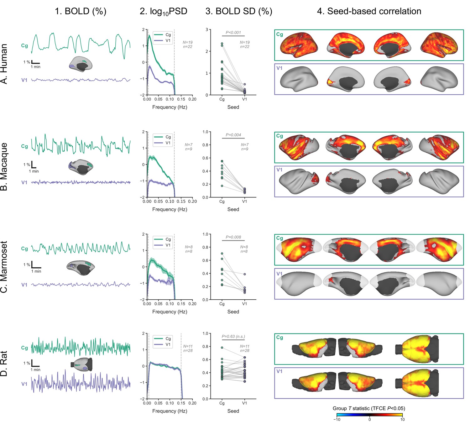
Primate V1 is uncoupled from the rest of the cortex during burst-suppression.
(A) Blood-oxygen-level-dependent (BOLD) signal time series extracted from two regions-of-interest, the cingulate (Cg) area 24cd and the primary visual cortex (V1), are shown for an example human subject during burst-suppression (A1). The power spectral density (PSD) of the two regions’ time series is plotted as mean ± SEM across all functional magnetic imaging (fMRI) runs with burst-suppression (A2). The SD of the time series is plotted for the same fMRI runs as a measure of BOLD signal amplitude (A3). The SDs of the two regions are compared using a paired samples two-tailed Wilcoxon rank-sum test (p values given). The results of seed-based correlation analysis—performed for each of the two regions—are shown overlaid on the cortical surface (A4). The group statistics were carried out with FSL randomise; the resulting T statistic maps were thresholded using threshold-free cluster enhancement (TFCE) and a corrected p<0.05. The other panels show the exact same plots as in A, but for macaques (B), marmosets (C), and rats (D), respectively. The cingulate (Cg) seed corresponds to the macaque area 24c, the marmoset area 24, and the rat primary cingulate cortex. Marmoset brain areas not covered by the fMRI volume are shown in white. The fMRI runs included in the analysis are the ones with an asymmetric PC, same as in previous figures. N: number of subjects; n: number of fMRI runs. The BOLD SD and PSD values across species and regions-of-interest are provided in Figure 6—source data 1. Figure 6—figure supplement 1 shows how the BOLD signal time series from the two regions vary across sevoflurane concentrations in anesthetized humans.
-
Figure 6—source data 1
BOLD SD and PSD values across species and regions-of-interest (numerical data for Figure 6 A2–D2 and A3–D3).
- https://cdn.elifesciences.org/articles/74813/elife-74813-fig6-data1-v1.xlsx
Figure 6—figure supplement 1
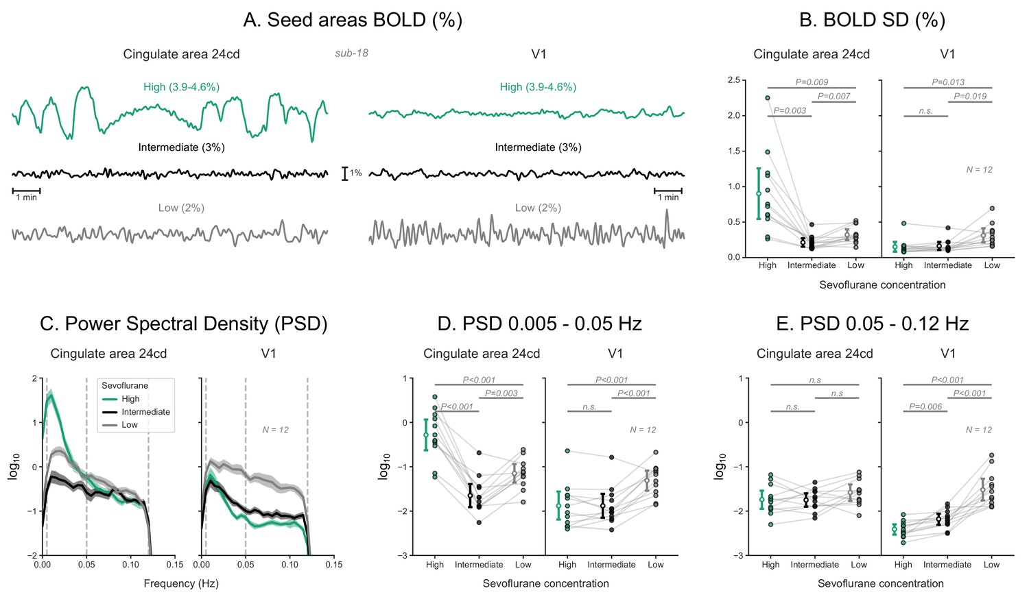
Blood-oxygen-level-dependent (BOLD) signal time series across sevoflurane concentrations in humans.
(A) BOLD signal time series extracted from two regions-of-interest—left cingulate area 24cd and left V1—of a human subject across three concentrations of sevoflurane anesthesia. (B) The SD of these time series are plotted as dots across 12 human subjects. The estimated least-squares means, with 95% confidence intervals, are plotted to the left of the dots. p values indicate the results of Tukey post-hoc pairwise comparisons following a repeated-measure ANOVA (sevoflurane concentration as the within-subject repeated measure). (C) For each region and sevoflurane concentration, the decadic logarithm of the BOLD signal’s power spectral density (log10PSD) is plotted as mean ± SEM across the 12 subjects. (D) Integrated log10PSD within a low (0.005–0.05 Hz) frequency range. (E) Integrated log10PSD within a high (0.05–0.12 Hz) frequency range. Estimated least-squares means, confidence intervals, and p values are shown as in panel B. N: number of subjects; n.s.: non-significant. Detailed results of repeated-measures ANOVAs and post-hoc tests are given in Figure 6—figure supplement 1—source data 1.
-
Figure 6—figure supplement 1—source data 1
Results of repeated-measures ANOVA and post-hoc pairwise tests for Figure 6—figure supplement 1.
- https://cdn.elifesciences.org/articles/74813/elife-74813-fig6-figsupp1-data1-v1.xlsx
Figure 7
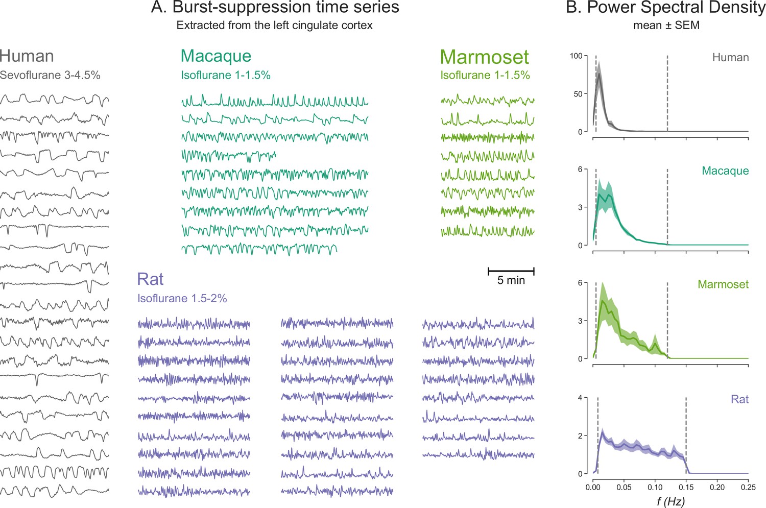
Burst-suppression timescales across species.
(A) Blood-oxygen-level-dependent (BOLD) functional magnetic resonance imaging (fMRI) signal time series extracted from the cingulate cortex are shown for all runs classified as burst-suppression across the four species. This region—also used for the seed-based analysis (see Figure 6)—was selected because of its strong correlation with burst-suppression (i.e., asymmetric principal components) in all species. The time series are shown min-max scaled to emphasize differences in time, not in amplitude. The time series peaks appear shorter in duration and occur more frequently as we move from humans to non-human primates and finally to rats. (B) This effect is reflected on the power spectral density (PSD) plots of the time series, with increasingly higher frequencies being present from top to bottom. PSD was computed from time series normalized to percent-signal-change (relative to the mean) prior to min-max scaling. Vertical dashed lines indicate the cutoffs of the bandpass filter that was used for fMRI preprocessing.
Tables
Table 1
Datasets of the present study.
For age and weight, mean and range values are reported. Anesthetic concentration refers to the range used during functional magnetic resonance imaging acquisition. In humans and macaques the measured end-tidal concentration of the anesthetic gas is reported, in marmosets and rats the output concentration of the vaporizer.
| Human | Macaque | Marmoset | Rat 1 | Rat 2 | |
|---|---|---|---|---|---|
| Species/Strain | - | M. fascicularis | C. jacchus | Wistar | Wistar |
| Site | Munich | Göttingen | Göttingen | Göttingen | Kuopio |
| Field strength | 3T | 3T | 9.4T | 9.4T | 7T |
| Subjects (N) | 20 | 13 | 21 | 11 | 6 |
| Sex | M | F | 11 F | F | M |
| Age (years) | 26 (20–36) | 13.7 (6.8–19.8) | 6.0 (1.9–14.2) | - | - |
| Body Weight | - | 5.4 kg (3.6–8.1) | 407 g (337–517) | 398 g (350–450) | 307 g (265–350) |
| Anesthetic | Sevoflurane | Isoflurane | Isoflurane | Isoflurane | Isoflurane |
| Concentration (%) | 2.0–4.6 | 0.95–1.50 | 0.6–1.1 | 1.5–2.5 | 1.3 |
Additional files
Download links
A two-part list of links to download the article, or parts of the article, in various formats.
Downloads (link to download the article as PDF)
Open citations (links to open the citations from this article in various online reference manager services)
Cite this article (links to download the citations from this article in formats compatible with various reference manager tools)
Spatial signatures of anesthesia-induced burst-suppression differ between primates and rodents
eLife 11:e74813.
https://doi.org/10.7554/eLife.74813


