Self-organization of in vitro neuronal assemblies drives to complex network topology
- Department of Biochemistry – Escola Paulista de Medicina – Universidade Federal de São Paulo (UNIFESP), Brazil
- Department of Psychological and Brain Sciences, Indiana University, United States
- Department of Informatics, Computing, and Engineering, Indiana University, United States
- Department of Physics, Indiana University, United States
- Department of Neurology and Neurosurgery – Escola Paulista de Medicina – Universidade Federal de São Paulo (UNIFESP), Brazil
Figures
Figure 1
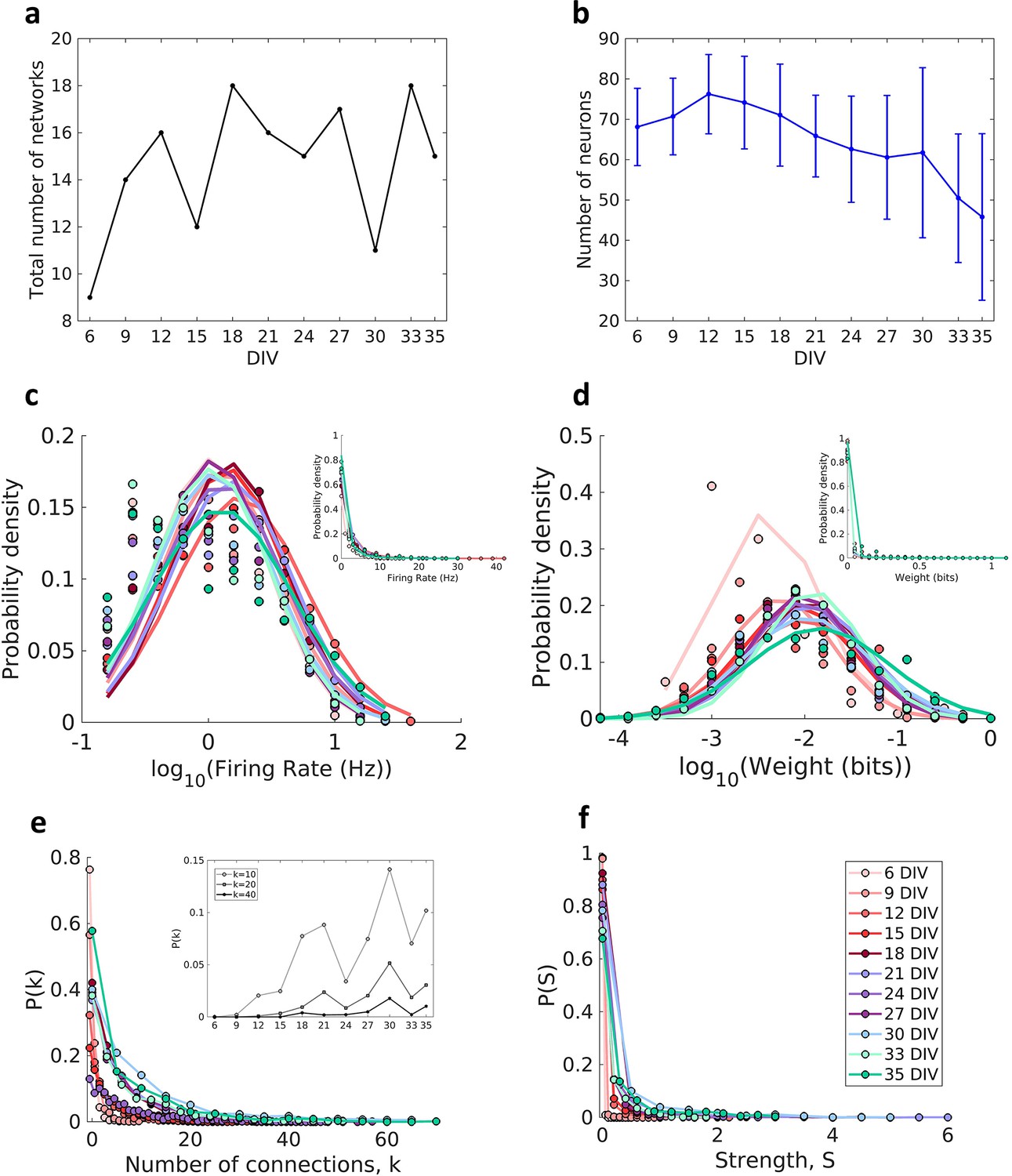
Description of the networks.
Neuronal cultures were recorded from 6 to 35 days in vitro (DIV). (a) Number of the total networks analyzed for each considered DIV. (b) Number of neurons recorded in the cultures for each DIV (mean ± SEM). Sample size for each DIV: 9, 14, 16, 12, 18, 16, 15, 17, 11, 18, and 15. (c) Distributions of the pooled logarithm firing rate of neurons recorded in each DIV represented by the Gaussian fit of the computed values. Neurons with a firing rate lower than 0.2 Hz were cut off. Inset: distributions of the pooled firing rate of neurons recorded in each DIV fitted by the generalized Pareto distribution. (d) Distributions of the pooled logarithm weights represented by the Gaussian fit of the normalized transfer entropy resulting from the significant connections (see Materials and methods). Inset: distributions of the pooled weight values computed in each DIV fitted by the generalized Pareto distribution. (e) Distributions of the pooled number of connections per neuron by DIV. Inset: probability of connections with k = 10, 20, and 40 for each DIV. (f) Distributions of the pooled strength were defined as the sum of the weights of the connections per neuron by DIV.
Figure 2 with 1 supplement

The relationship between the weight of effective connection and the distance between neurons.
(a) Joint probability distributions of the pooled logarithm weight and the distance between neurons. Weights were defined as the normalized transfer entropy resulting from significant connections while distance was calculated as the Euclidean distance between the electrodes from where the two neurons involved in a connection were recorded. (b) Mean probability density by distance. (b–d) Each row relates to 6, 12, 18, 24, 30, and 35 days in vitro (DIV), respectively. (c) Probability density only for 25 µm of the distance between neurons for each connection weight (logarithm). (d) Probability density only for 1425 µm of the distance between neurons for each connection weight (logarithm). Statistical tests: Kruskal-Wallis test followed by the Tukey-Kramer post-hoc test. (e) Distance between neurons over DIV (mean ± SEM). Sample size for each DIV: 4, 13, 16, 12, 18, 16, 15, 17, 11, 18, and 11. Asterisks indicate p-values ≤ 0.05 (*).
Figure 2—figure supplement 1
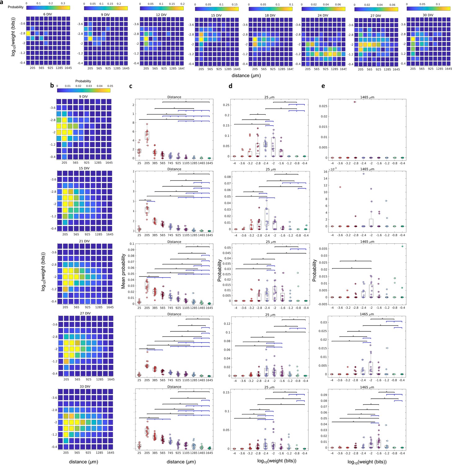
The relationship between the weight of effective connection and the distance between neurons.
(a) Joint probability distributions of the logarithm weight and the distance between neurons for Culture 1 over the days in vitro (DIV) that the culture was recorded. Weights were defined as the normalized transfer entropy resulting from significant connections while distance was calculated as the Euclidean distance between the electrodes from where the two neurons involved in a connection were recorded. (b) Joint probability distributions of the pooled logarithm weight and the distance between neurons. (b–e) Each row relates to 9, 15, 21, 27, and 33 DIV, respectively. (c) Mean probability density by distance. (d) Probability density only for 25 µm of the distance between neurons for each connection weight (logarithm). (e) Probability density only for 1425 µm of the distance between neurons for each connection weight (logarithm). Statistical tests: Kruskal-Wallis test followed by the Tukey-Kramer post-hoc test. Asterisks indicate p-values ≤ 0.05 (*).
Figure 3
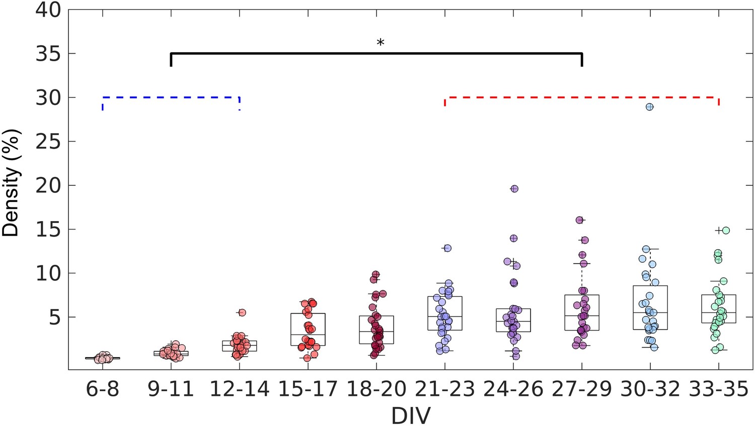
Evolution of the edge density of effective networks over time.
Edge density was computed by normalizing the number of actual connections by the total number of possible connections (N2–N, where N is the total number of nodes). The edge density per period was defined as the median for each culture (28 cultures) among 3 days. Statistical tests: Kruskal-Wallis test followed by the Tukey-Kramer post-hoc test. Asterisk indicates p-value ≤ 0.05 (*).
Figure 4
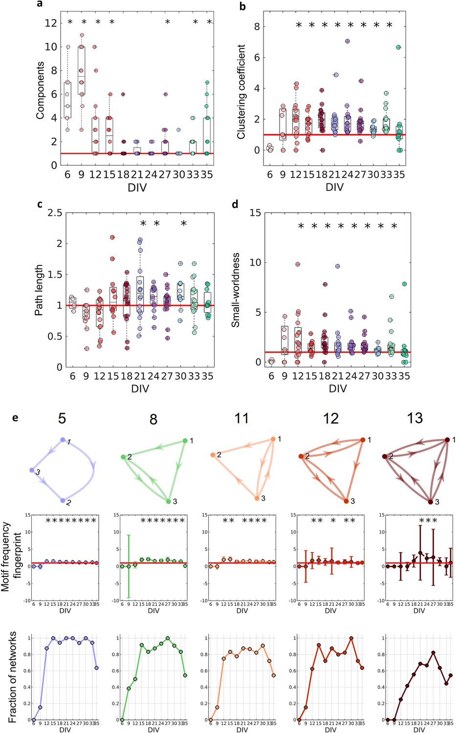
Graph-theoretic measures over maturation.
Various network measures were computed from effective networks in different periods of maturation. (a) Number of components computed for each network by days in vitro (DIV). The red line represents the convergence of the entire network to only one large and fully connected component. (b, c) Global clustering coefficient, and path length, respectively. The results for both coefficients in actual networks were normalized by the average result from 100 randomized networks (see Null model in the Materials and methods section). The red line represents when the normalization is equal to 1 meaning the results for actual and random networks are the same. (d) Small-worldness results considering the actual clustering coefficient and path length compared to a random network. The red line represents that the network architecture is not a small-world. (e) Motifs that were found significantly more frequent than in random networks during maturation. The motif frequency fingerprint was considered as the total motif frequency of occurrence in the whole network; results were normalized by the same measures in random networks (values are presented as mean ± SEM). The red line represents where the frequency of the motif is the same as in random networks. The fraction of networks was computed by dividing the number of networks that presented the motif by the total number of networks that presented at least one motif. Sample size for each DIV: 4, 13, 16, 12, 18, 16, 15, 17, 11, 18, and 11. To test whether the results come from a population with a median equal to 1 the Wilcoxon signed-rank test was used. Asterisks indicate p-values ≤ 0.05 (*).
Figure 5
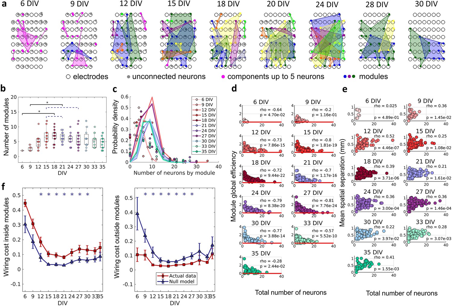
The emergence of modular organization.
A community detection algorithm allowed to track the division of the networks into non-overlapping modules. (a) Schematic representation of the physical location of modules in culture over days in vitro (DIV). Connected and colored areas link the neurons within the same modules. (b) Mean number of modules for each network by DIV. Statistical tests: Kruskal-Wallis test followed by the Tukey-Kramer post-hoc test. (c) Distributions of the pooled number of neurons by module represented by the Poisson fit of the computed values by DIV. (d) Global efficiency was computed for each module and normalized by the averaged coefficient considering the same neurons in 100 random networks (see Null model in the Materials and methods section). The values shown are the pooled normalized coefficients for all the modules in all cultures for the same DIV. The red line represents where the module’s global efficiency is the same as in random networks. The correlation between the module’s global efficiency and the total number of neurons per module was calculated by using Spearman’s rho. (e) Spatial separation was computed by averaging the length of all connections within each module. The connection length was calculated by the Euclidean distance between the electrodes that gathered the signal from the two neurons involved in each connection. The values shown are for all modules in each culture per DIV. The correlation between the spatial separation and the total number of neurons per module was calculated by using Spearman’s rho. (f) Wiring cost computation was performed by summing up the Euclidean distance of the electrodes that gathered the signals from the two neurons related to each connection. Results for actual networks are presented as mean ± SEM considering the connection inside and outside modules normalized by the total wiring cost of the network separately. Additionally, results for the null model were averaged from 100 random networks, taking the same neurons for each module but different connections. Sample size for each DIV: 4, 13, 16, 12, 18, 16, 15, 17, 11, 18, and 11. Actual and modeled results were compared on the same DIV by using the ANOVA. Asterisks indicate p-values ≤ 0.05 (*).
Figure 6
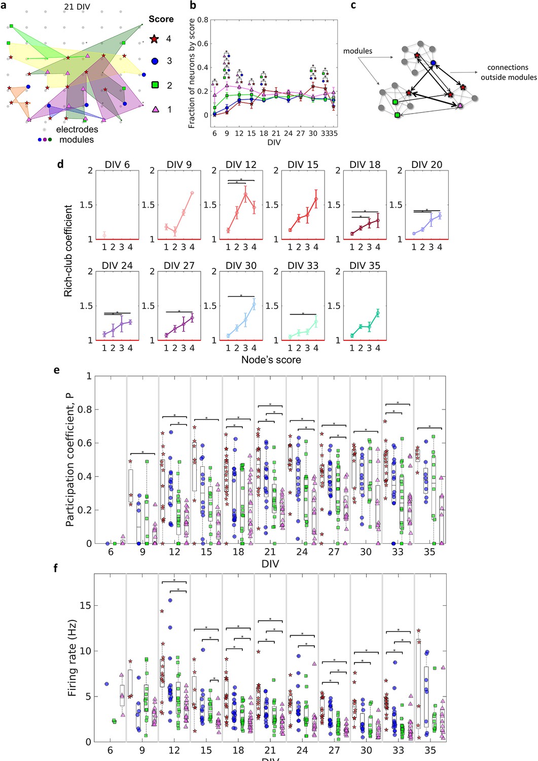
Topologically important nodes and their role as module integrators.
Neuron hubness was classified by scores. Four measures were computed for each neuron, degree, strength, betweenness centrality, and closeness centrality. The score of a neuron was based on the number of measures that it ranked in the highest values.(a) Graphical representation of the location of nodes with different scores in one culture after 21 days in vitro (DIV). (b) Evolution of the fraction of neurons by score, defined as the number of neurons for each score normalized by the total number of neurons in the culture, over DIV. Results are presented as mean ± SEM, they were compared on the same DIV by using the one-way ANOVA. (c) Graph representation of outside modules connections used in the weighted rich-club coefficient computation. Black arrows represent the connections used. (d) Weighed rich-club coefficient computed considering only the connections highlighted in c. Values are presented as the mean ± SEM for actual networks normalized by the average value for 100 random networks, where the same neurons but different connections were considered. The red line represents where the rich-club coefficient is the same as in random networks. (e) Mean participation coefficient for neurons with each score in every culture over DIV. (f) Mean firing rate for neurons with each score in every culture over DIV. Sample size for each DIV by score: 6 DIV {4: 0; 3: 1; 2: 2; 1: 4}; 9 DIV {4: 3; 3: 6; 2: 13; 1: 13}; 12 DIV {4: 13; 3: 15; 2: 16; 1: 16}; 15 DIV {4: 7; 3: 12; 2: 12; 1: 12}; 18 DIV {4: 18; 3: 18; 2: 18; 1: 18}; 21 DIV {4: 14; 3: 16; 2: 16; 1: 16}; 24 DIV {4: 11; 3: 14; 2: 15; 1: 15}; 27 DIV {4: 14; 3: 17; 2: 17; 1: 16}; 30 DIV {4: 10; 3: 11; 2: 10; 1: 11}; 33 DIV {4: 15; 3: 16; 2: 18; 1: 18}; 35 DIV {4: 5; 3: 8; 2: 10; 1: 11}. Statistical tests: Kruskal-Wallis test followed by the Tukey-Kramer post-hoc test. Asterisks indicate p-values ≤ 0.05 (*).
Figure 7

Comparison of hypotheses on the emergence of Small-world architecture.
Alternative scenarios that might support the development of networks into highly clustered nodes reached by a small number of steps. Watts and Strogatz, 1998 firstly suggested that a random rewiring of a few edges in a lattice network can lead it to a small-world organization. Kwok et al., 2007 adapted this hypothesis to the context of neuroscience, suggesting that neurons are initially randomly connected, and these connections are rewired by comparing the synchronization of one neuron to the entire network. Following a Hebbian rewiring rule, highly synchronized neurons receive or maintain a connection while unsynchronized neurons lose it, also leading the network to a small-world organization after a few steps of rewiring. Both hypotheses were raised in a computational model environment, however, the rewiring scenario would involve a high amount of time, wiring cost, and energy to take place in the brain. Considering the results from empirical data reported herein and the silent synapses activation evidence, we hypothesized that neurons might initially make silent synapses with nearby neurons and only synapses between synchronized neurons would be activated. Thus, considering 3 neurons A, B, and C connected by silent synapses. If the synapse between neurons A and B is activated, because they have a synchronized firing activity and the same occurs for neurons A and C. Likely, neurons B and C would also have a synchronized firing activity turning on the synapse between them. The activation of a significant number of synapses gives rise to a Small-world topology in effective networks by a mechanism of selection of structural connections instead of a rewiring process.
Figure 8
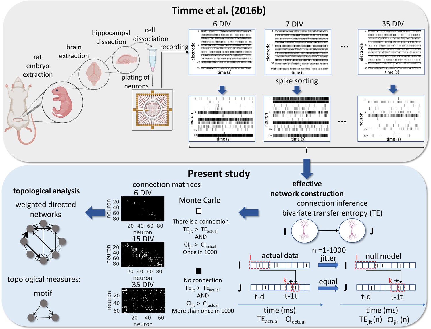
Experimental and data analysis procedure.
Top row, left to right, bottom row, right to left. In the work of Timme et al., 2016a brains were extracted from embryos on gestational day 18. The hippocampi were dissected from the rest of the neuronal tissue and the hippocampal neurons were dissociated and plated on a multi-electrode array (MEA). The cultures were recorded from 6 to 35 days in vitro (DIV). The signals from the 60 electrodes were spike-sorted to reconstruct a binned and binary time series for each neuron. From this data set, we constructed effective networks, by applying a transfer entropy (TE) bivariate analysis. To infer a connection from a neuron I to a neuron J we computed the TE for each delay ranging from 1 to 20ms. Taking the highest value as the TEactual and the considered areas of the TE result curve in function of delays as the CIactual. The time series of neuron I was jittered and the TEjit(n) and CIjit(n) were calculated following the same steps for actual data with n ranging from 1 to 1000. Connection matrices were constructed using a Monte Carlo approach by comparing how many times the TE results for the null model were higher than the result for actual data. The resulting weighted directed networks were constructed by normalizing the TEactual value of the connections considered significant by the entropy of the neuron J. Finally, we analyzed the progression of the topology of these networks over time.
Additional files
Download links
A two-part list of links to download the article, or parts of the article, in various formats.
Downloads (link to download the article as PDF)
Open citations (links to open the citations from this article in various online reference manager services)
Cite this article (links to download the citations from this article in formats compatible with various reference manager tools)
Self-organization of in vitro neuronal assemblies drives to complex network topology
eLife 11:e74921.
https://doi.org/10.7554/eLife.74921


