A neural mechanism for detecting object motion during self-motion
- Department of Biomedical Engineering, Sungkyunkwan University, Republic of Korea
- Department of Brain and Cognitive Sciences, Center for Visual Science, University of Rochester, United States
- Center for Neuroscience Imaging Research, Institute for Basic Science, Republic of Korea
- Center for Neural Science, New York University, United States
Figures
Figure 1 with 3 supplements

Object detection task and behavior.
(A) Schematic illustration of the moving object detection task. Once the animal fixated on a center target, objects were presented while the animal experienced self-motion. Saccade targets then appeared at the center of each object, and the animal indicated the dynamic object (moving relative to the scene) by making a saccade. (B) Schematic illustration of stimulus generation from behind and above the observer. A stationary far object that lies within the neuron’s receptive field (RF, dashed circle) has rightward image motion when the observer moves to the right. The other (dynamic) object moves rightward independently in space (cyan arrow) such that the object’s net motion suggests a far depth while binocular disparity cues suggest a near depth. Gray shaded region indicates the display screen; cross indicates the fixation point. (C) Average behavioral performance across recording sessions for each animal (n=47 sessions from monkey 1 [M1] and n=57 sessions from monkey 2 [M2], excluding two sessions for which the standard set of ΔDepth values was not used). Error bars denote 95% CIs. (D) Normalized regression coefficients for depth from disparity (βBD), depth from motion parallax (βMP), and ΔDepth (βΔ) are shown separately for chosen locations and not-chosen locations (see text for details). Gray and black bars denote data for M1 (n=44) and M2 (n=53), respectively. (E) Proportion of fits for which each regression coefficient was significantly different from zero (alpha = 0.05). Format as in panel D.
Figure 1—figure supplement 1
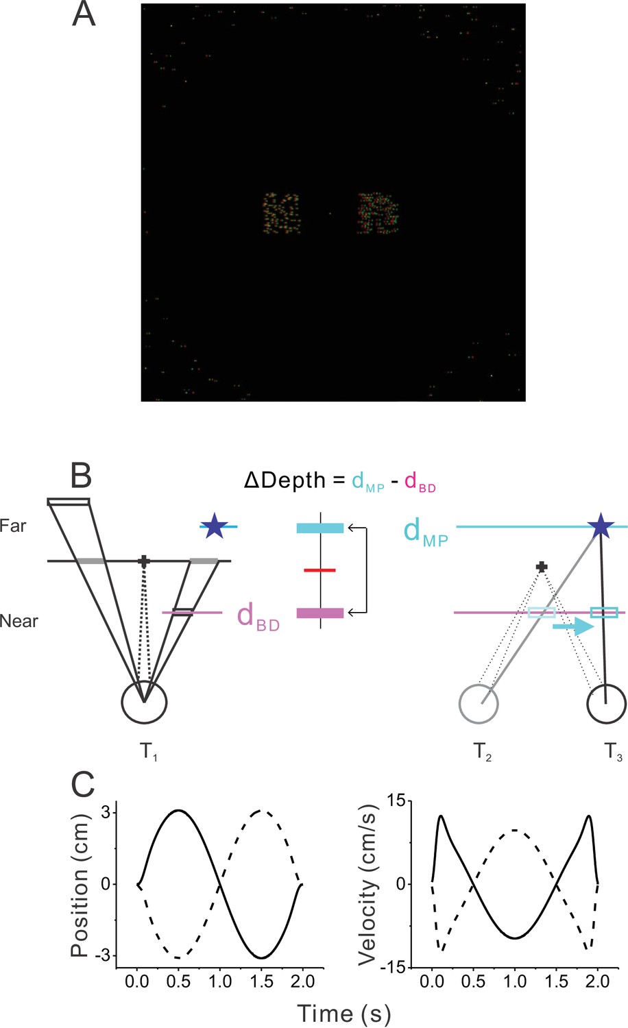
Visual display and motion trajectories.
(A) A screen shot of the visual stimulus. It consisted of fixation target at the center, two or four objects (two objects shown), and background dots, which were masked within the central region of the display. Red and green dots represent images shown to the left and right eyes. (B) Schematic drawing (top view) depicting the rendering geometry for a far stationary object (left) and a near dynamic object (right). Left: the location of a stationary object was initially defined by the horizontal and vertical coordinates on the screen and then was ray-traced onto a virtual plane located at the depth of the object. A moving object was initially positioned at the depth defined by binocular disparity (dBD, cyan) in the same way as the stationary object. The location of the object at a different depth (dMP) was ray-traced (blue star). Right: once the self-motion trajectory of the animal was determined, the location of the virtual object (blue star) was ray-traced onto the plane defined by binocular disparity (dBD) to compute the trajectory of independent movement at dBD. The resultant retinal motion mimics motion parallax at depth dMP. We used the depth difference (ΔDepth) to manipulate the difficulty of the task. (C) Time courses of position (left) and velocity (right) of the animal during the modified sinusoidal translational motion (see Methods for details).
Figure 1—figure supplement 2
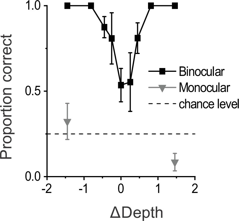
Results from a control experiment including monocularly presented objects.
Psychometric data are shown from control experiments (n=3 sessions, 1180 total trials) in which dynamic and stationary objects were shown with (binocular) and without (monocular) disparity cues. These data were collected in the version of the task with four objects (see also Figure 1—figure supplement 3), such that chance level performance was 25% (dashed horizontal line). Monocular conditions were only presented for the largest (easiest) ΔDepth values (16% of total trials). While performance in the binocular condition shows a robust V-shaped curve similar to the main dataset (Figure 1C), performance in the monocular condition is very poor. Error bars represent 95% CIs.
Figure 1—figure supplement 3
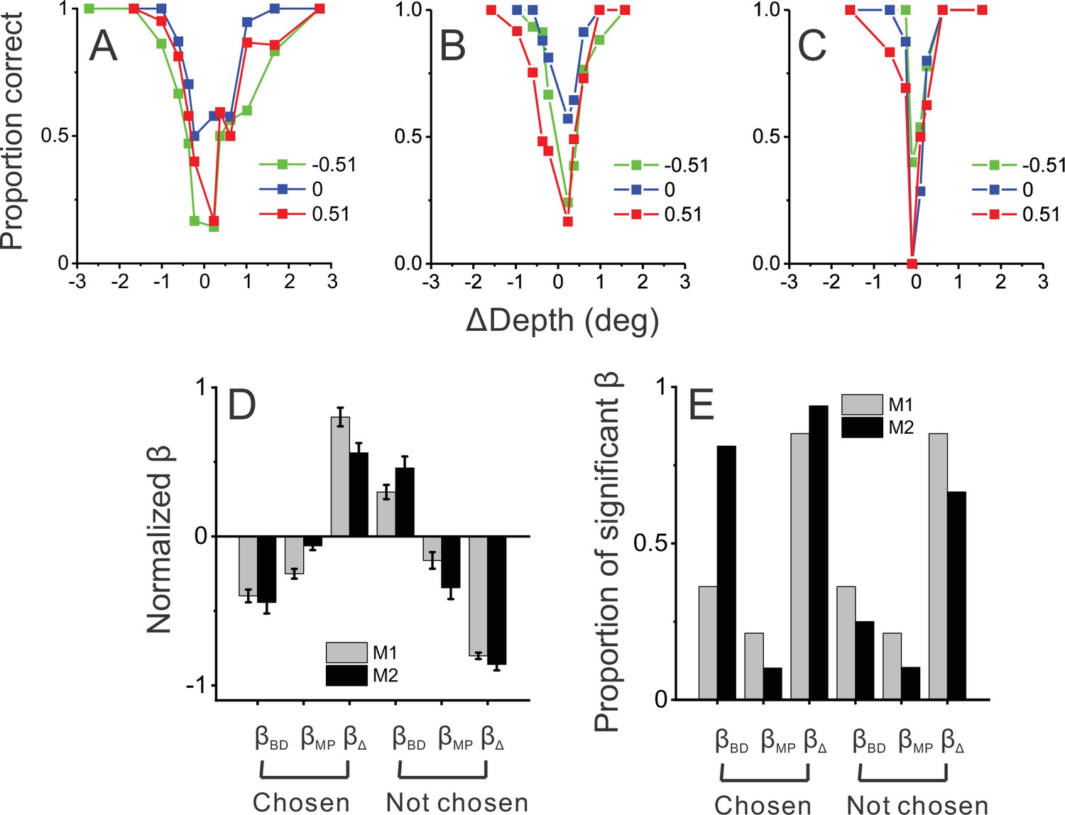
Behavioral performance in the more generalized task with four objects.
(A) An example session from monkey 1 (M1) in which the animal performed the detection task with four objects and three pedestal depths (red, green, and blue colors). (B) An example session from monkey 2 (M2) prior to neural recordings. (C) Another example session from M2 after neural recording experiments were completed. (D) Normalized beta coefficients from logistic regression analysis for the four-object task; format as in Figure 1D. Data include 35 sessions from M1 from before neural recordings, 27 sessions from M2 from before neural recordings, and 10 sessions from M2 after neural recordings. (E) Proportion of beta coefficients that are significantly different from zero. Format as in Figure 1E.
Figure 2 with 1 supplement
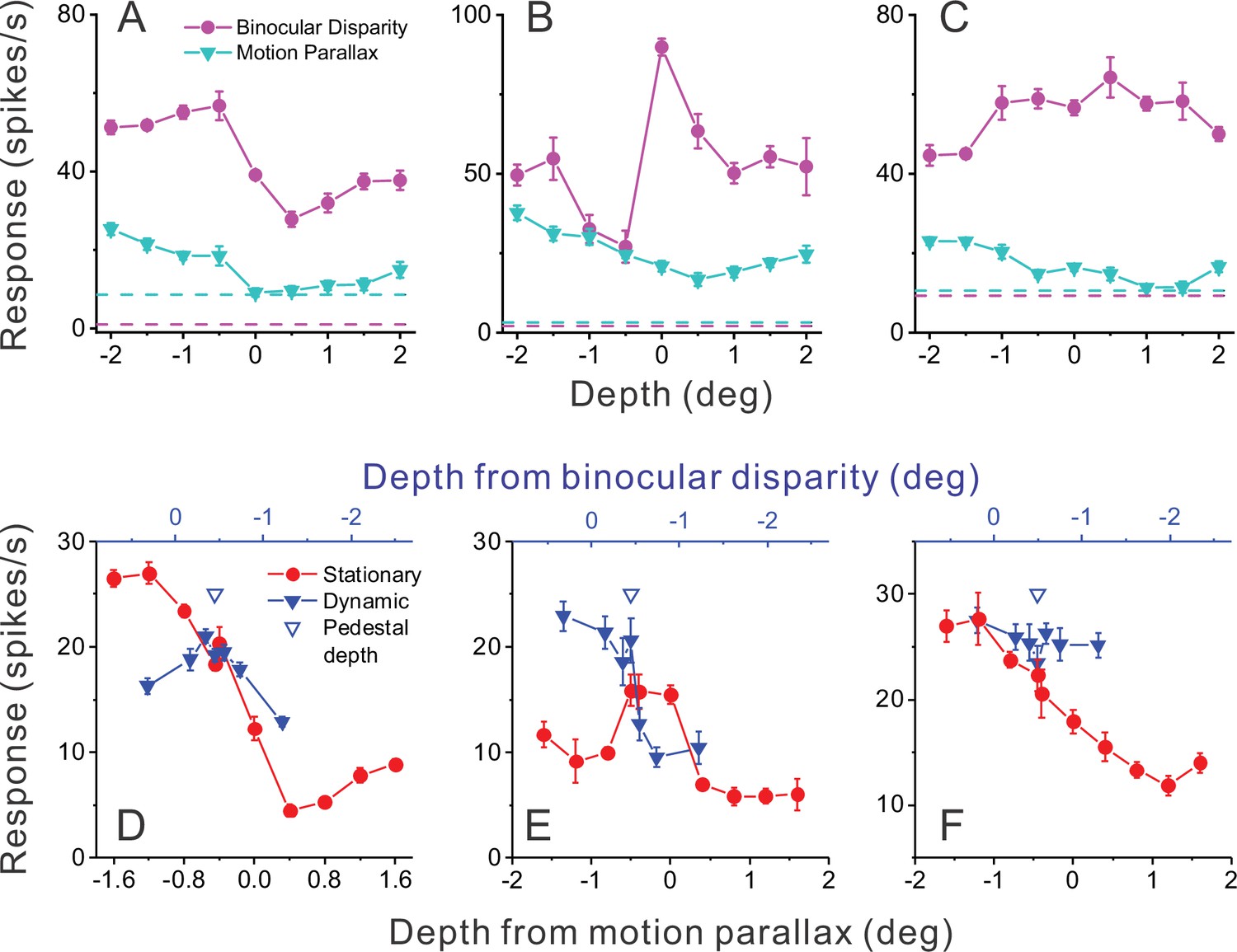
Responses of representative MT neurons.
(A) Depth tuning curves for an example ‘congruent’ neuron preferring near depths based on both binocular disparity (magenta) and motion parallax (cyan) cues (DSDIBD = −0.81; DSDIMP = −0.70 [DSDI, depth-sign discrimination index]; p<0.05 for both, permutation test; correlation RMP_BD = 0.76, p=0.016). Dashed horizontal lines indicate baseline activity for each tuning curve. (B) Tuning curves for an example ‘opposite’ neuron preferring small far depths based on binocular disparity but preferring near depths based on motion parallax (DSDIBD = 0.41; DSDIMP = −0.67; p<0.05 for both, permutation test; RMP_BD = −0.36, p=0.32). (C) Another example opposite cell preferring far depths based on binocular disparity but near depths based on motion parallax (DSDIBD = 0.46; DSDIMP = −0.56; p<0.05 for both, permutation test; RMP_BD = −0.73, p=0.025). (D) Responses of the neuron in panel A to stationary objects (red) and dynamic objects (blue) during performance of the detection task. Stationary objects were presented at various depths (bottom abscissa). Dynamic objects generally have conflicts (ΔDepth ≠ 0) between depth from motion parallax (bottom abscissa) and binocular disparity (top abscissa). The pedestal depth at which ΔDepth = 0 is shown as an unfilled blue triangle. (E) Responses during the detection task for the opposite cell of panel B. Format as in panel D. (F) Responses during detection for the neuron of panel C. Error bars in all panels represent s.e.m.
Figure 2—figure supplement 1
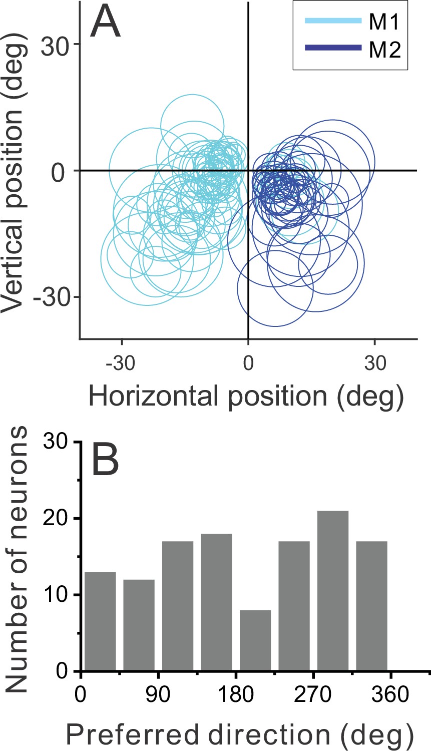
Distribution of receptive field (RF) properties.
(A) Positions and sizes of the RFs of our sample of MT neurons (n=123). Each circle represents the contour of the RF, defined as the center and diameter obtained from the RF mapping and size tuning protocols (see Methods). (B) Distribution of preferred directions for the sample of neurons (n=123), where 0 deg corresponds to rightward motion and 90 deg corresponds to upward motion.
Figure 3
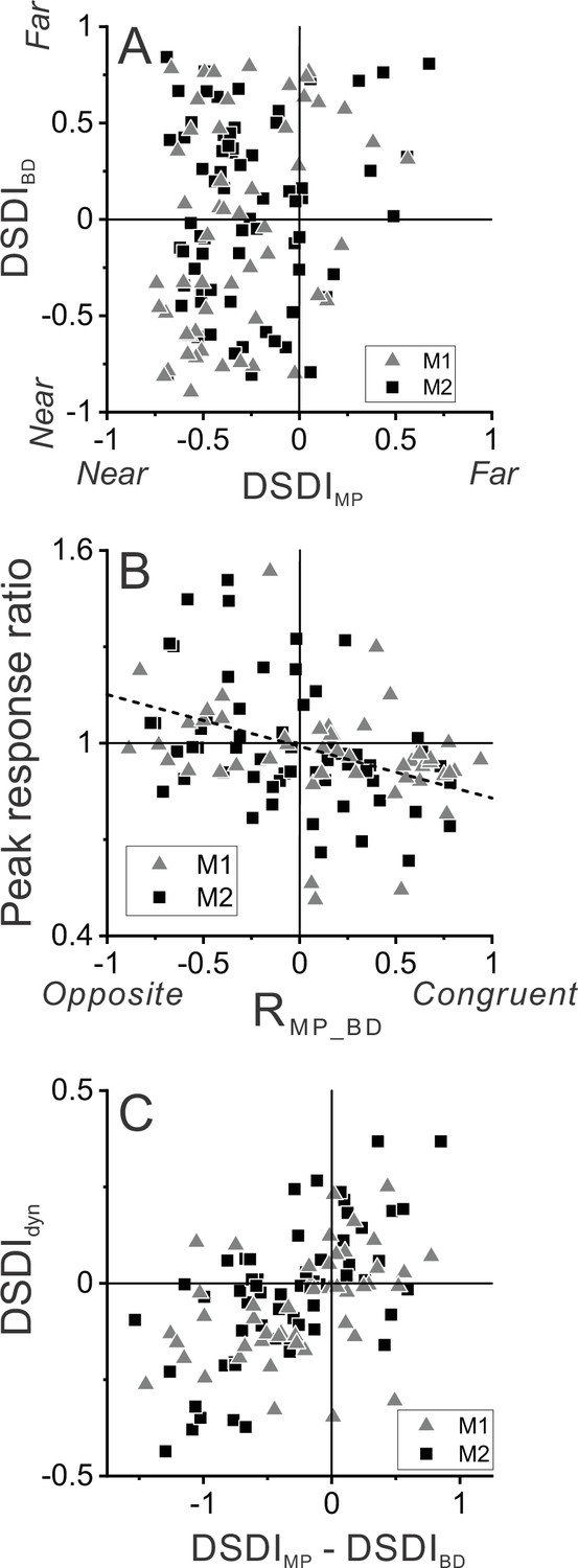
Relationship between selectivity for moving objects and congruency between depth cues.
(A) Population summary of congruency of depth tuning for disparity and motion parallax. The depth-sign discrimination index (DSDI) value for binocular disparity tuning (DSDIBD) is plotted as a function of the DSDI value for motion parallax tuning (DSDIMP) for each neuron (n=123). Triangles and squares denote data for monkey 1 (M1) (n=53) and monkey 2 (M2) (n=70), respectively. (B) Population summary of relationship between relative responses to dynamic and stationary objects as a function of depth tuning congruency. The ordinate shows the ratio of peak responses for dynamic:stationary stimuli. The abscissa shows the correlation coefficient (RMP_BD) between depth tuning for motion parallax and disparity. Dashed line is a linear fit using type 2 regression (n=106; n=47 from M1 and n=59 from M2; sample includes all neurons for which we completed the detection task). (C) Population summary (n=106) of the relationship between the preference for ΔDepth of the dynamic object (as quantified by DSDIdyn, see Methods) and the difference between DSDIMP and DSDIBD.
Figure 4 with 1 supplement

Relationship between MT responses and detection of object motion.
(A) When ΔDepth = 0, two stationary objects at the pedestal depth had identical retinal motion and depth cues. Animals still were required to report one of the objects as dynamic. (B) To compute detection probability (DP), responses to the ΔDepth = 0 condition were z-scored and sorted into two groups according to the animal’s choice. Filled and open bars show distributions of z-scored responses of an example MT neuron when the animal reported that the moving object was in and out of the receptive field (RF), respectively. (C) Distribution of DP values for a sample of 92 MT neurons, including all neurons tested in the detection task for which the animal made at least five choices in each direction (see Methods). Arrowhead shows the mean DP value of 0.56, which was significantly greater than 0.5 (p=6.0×10⁻⁵, n=92, t-test).
Figure 4—figure supplement 1
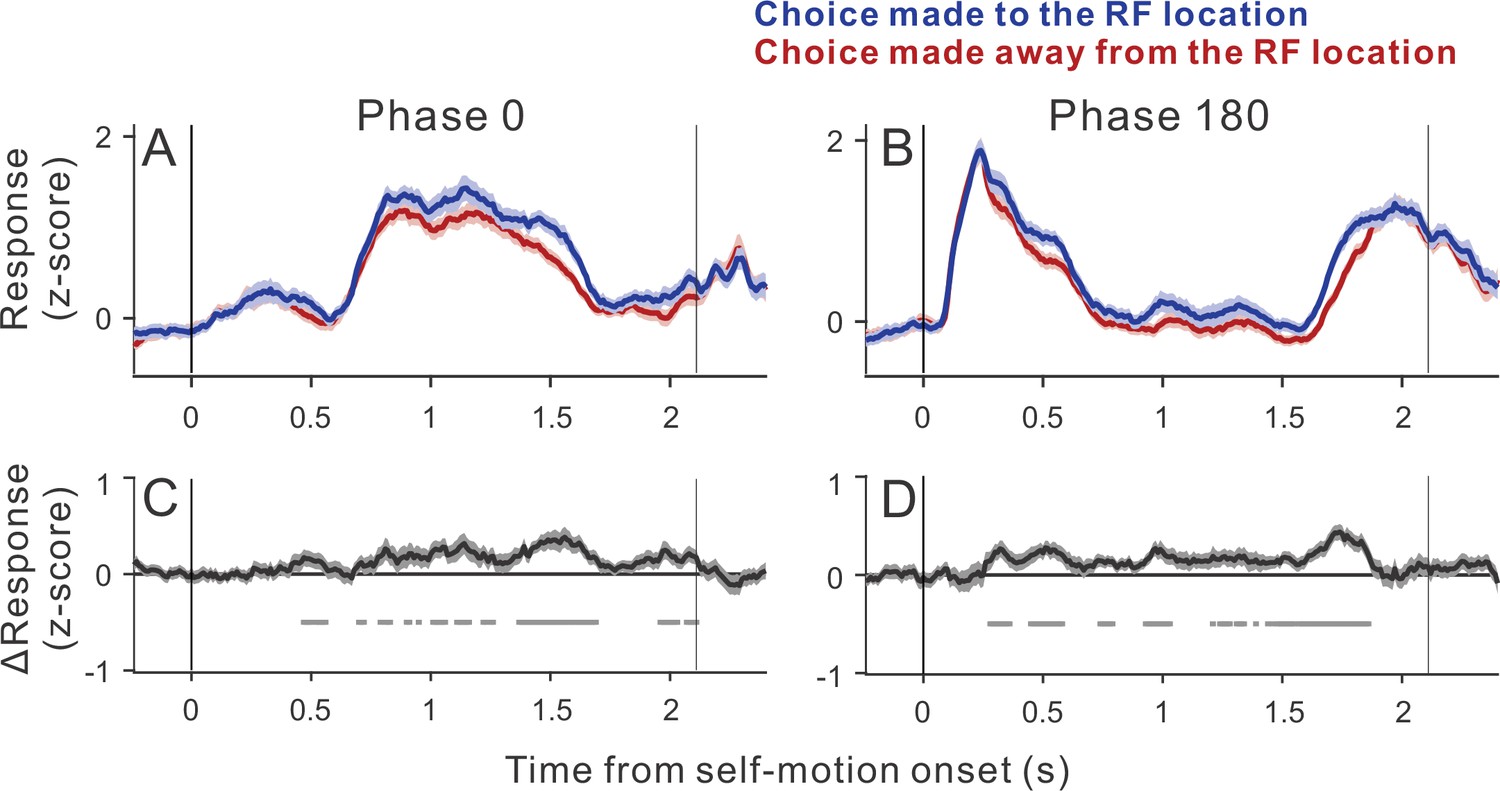
Time courses of choice-related activity.
Average population responses in the ambiguous trials (ΔDepth = 0) sorted by the animal’s choice. Neurons showing positive detection probability values were analyzed (n=64 neurons). (A) Average time courses of z-scored responses for the subset of trials in which self-motion began toward the neuron’s preferred direction (phase 0). We first computed the moving averages of spiking activity (150 ms window) for each neuron. The results were then z-scored based on the mean and SD of the moving averages for each neuron. (B) Responses when self-motion began toward the neuron’s anti-preferred direction (phase 180). (C) The differential response between the two choice groups shown in panel A. Gray marks denote time points at which the differential response is significantly different from zero (alpha = 0.05, n=64, Wilcoxon signed-rank test). (D) Differential response between the two choice groups shown in panel B. Shadings represent s.e.m.
Figure 5 with 1 supplement

Relationship between detection probability (DP) and neurometric performance for dynamic objects.
(A) Responses of an example opposite neuron to dynamic and stationary objects during the detection task. Format as in Figure 2D. (B) ROC values comparing responses to a dynamic object at each value of ΔDepth with responses to stationary objects, for the neuron of panel A. Neurometric performance (NP = 0.78 for this neuron) is defined as the average ROC area for all ΔDepth ≠ 0. (C) Distribution of z-scored responses sorted by choice for the same neuron as in panels A,B. Format as in Figure 4B. (D–F) Data from an example congruent cell, plotted in the same format as panels A–C. (G) Relationship between DP and NP for a population of 92 MT neurons. Dashed line: linear fit using type 2 regression (slope = 1.06, slope CI = [0.80 1.48]; intercept = –0.04, intercept CI = [–0.31 0.11]).
Figure 5—figure supplement 1
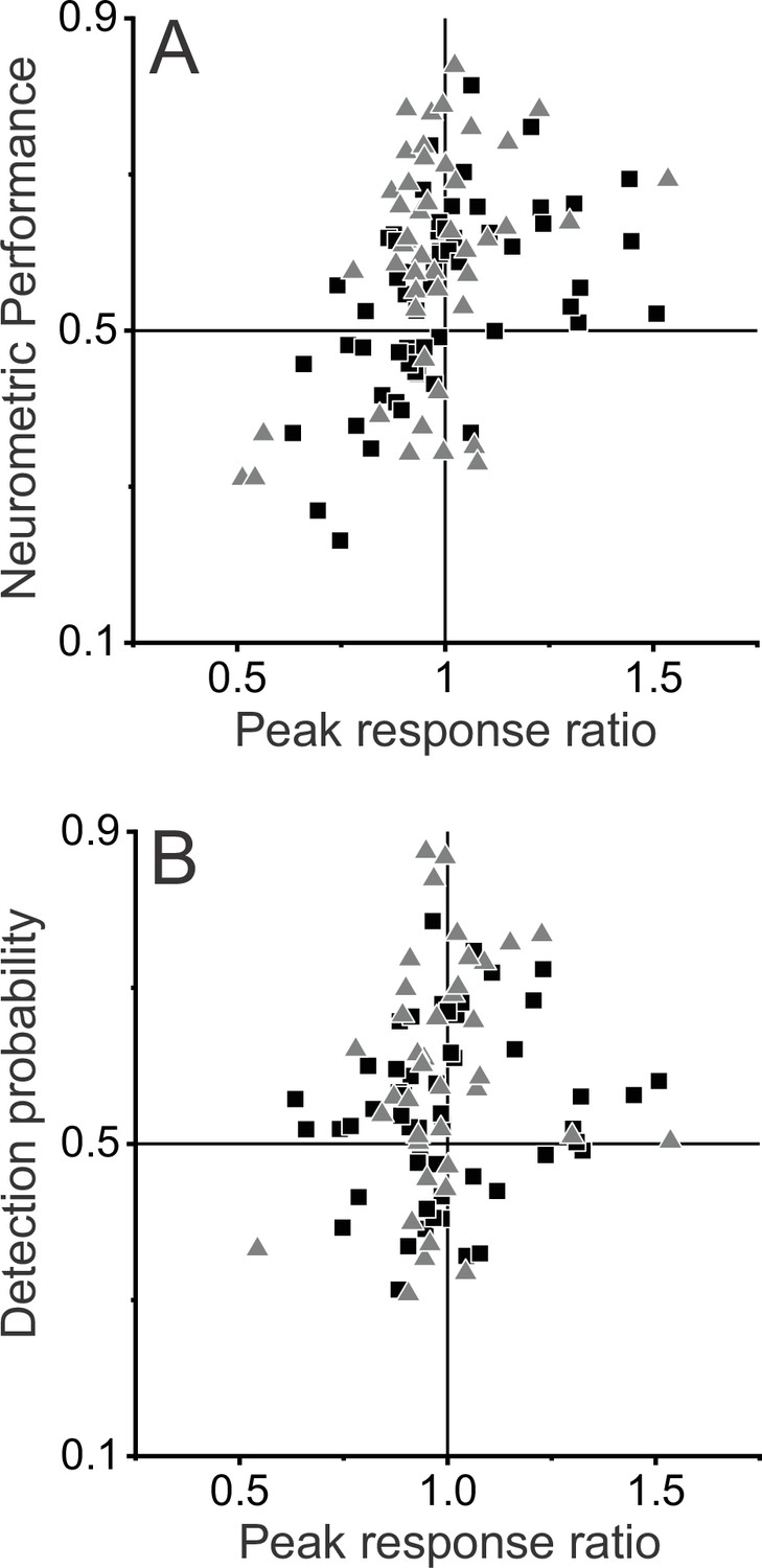
Relationships between preference for dynamic objects, neurometric performance (NP), and detection probability (DP).
(A) NP is plotted as a function of peak response ratio (dynamic:stationary objects). Triangles and squares denote data for monkey 1 (M1) (n=47) and monkey 2 (M2) (n=59), respectively. NP is significantly correlated with peak response ratio (R=0.43, p=4.5×10⁻⁶, Spearman rank correlation), such that neurons with greater peak response ratios tend to have greater NP. (B) DP is plotted as a function of peak response ratio for the subset of 92 neurons for which DP values could be computed (M1: n=39; M2: n=53). The positive trend in this relationship did not reach significance (R=0.12, p=0.25).
Figure 6

Linear decoding reproduces the relationship between detection probability (DP) and neurometric performance (NP).
(A) Performance of a linear decoder that was trained to detect moving objects based on simulated population responses with independent noise (see Methods for details). Error bars represent 95% CIs (n=100 simulations). (B) Neural responses were sorted by the output of the decoder to compute a predicted DP (DPpred) for each unit in the simulated population (n=97, including all neurons recorded in the detection task using identical ΔDepth and stationary depth values, see Methods). DPpred is plotted as a function of the measured NP for each neuron. Error bars represent 95% CIs (n=100 simulations). (C) Relationship between DPpred and the readout weight (β) for each unit in the decoded population. Error bars represent 95% CIs. (D–F) Analogous results for a decoder that was trained based on population responses with modest correlated noise (see text and Methods for details). Format as in panels A-C.
Figure 7

Decoder performance depends on selectivity for dynamic objects.
Decoding was performed separately for three subgroups of MT neurons based on their peak response ratios: lowest third (n=33), middle third (n=32), and highest third (n=32) of peak response ratio values. In addition, decoding was performed for mixed subgroups of the same size (n=32) that were selected randomly from the population. (A) Decoder performance for each subgroup based on peak response ratio. For each subgroup, 500 decoding simulations were performed (gray dots) using different samples of correlated noise, as described in Methods. For the mixed subgroup, each of the 500 simulations also involved drawing (without replacement) a new random subset of 32 neurons from the population. Black filled symbols denote mean proportion correct across the 500 simulations, and error bars represent 95% CIs. (B) Predicted detection probability (DPpred) for each neuron in each subgroup (gray symbols), along with mean DPpred values (black symbols, error bars denote s.e.m). For the mixed subgroup, data are shown for all 97 neurons since each neuron was included in many different subsamplings. In this case, gray data points represent the mean DPpred value for all random subsamplings (165, on average) that included each neuron. Median DPpred was not significantly different from 0.5 for the lowest third subgroup (p=0.59, n=33), was marginally significant for the middle third subgroup (p=0.043, n=32), and was significantly greater than 0.5 for the highest third (p=2.2×10⁻⁵, n=32) and mixed (p=3.2×10⁻⁵, n=97) subgroups (signed-rank tests comparing median DPpred with 0.5).
Videos
Video 1
Visual stimuli used in the dynamic object detection task.
Examples of visual stimuli in the two-object task, assuming that the receptive field of a neuron is located on the horizontal meridian. The video shows a sequence of seven stimuli, which are sorted by their ΔDepth values (ΔDepth = −1.53, −0.57, −0.21, 0, 0.21, 0.57, and 1.53 deg). The depth of the stationary object in each stimulus is labeled and was chosen randomly. In the actual experiment, the fixation target was stationary in the world, and the motion platform moved the animal and screen sinusoidally along an axis in the fronto-parallel plane (here a horizontal axis). Thus, the video shows the scene from the viewpoint of the moving observer. The stimulus sequences are equivalent to a situation in which the observer remains stationary, and the entire scene is translated in front of the observer. For each ΔDepth value, two full cycles of the stimulus are shown for display purposes; in the actual experiment, each trial consisted of just one cycle. During the second cycle of each stimulus in the video, the text label indicates whether the dynamic object was on the left or right side of the display. Red and green dots in the video denote the stereo half-images for the left and right eyes. Note that, without viewing the images stereoscopically and tracking the fixation target, it is generally not possible to determine the location of the dynamic object from the image motion on the display.
Additional files
Download links
A two-part list of links to download the article, or parts of the article, in various formats.
Downloads (link to download the article as PDF)
Open citations (links to open the citations from this article in various online reference manager services)
Cite this article (links to download the citations from this article in formats compatible with various reference manager tools)
A neural mechanism for detecting object motion during self-motion
eLife 11:e74971.
https://doi.org/10.7554/eLife.74971


