Long-term transverse imaging of the hippocampus with glass microperiscopes
- Interdepartmental Graduate Program in Dynamical Neuroscience, University of California, United States
- Department of Molecular, Cellular, and Developmental Biology, University of California, United States
- Cognitive and Systems Neuroscience Group, University of Amsterdam, Netherlands
- Neuroscience Research Institute, University of California, United States
- Department of Psychological and Brain Sciences, University of California, United States
- Department of Electrical and Computer Engineering, University of California, Santa Barbara, United States
Figures
Figure 1 with 2 supplements
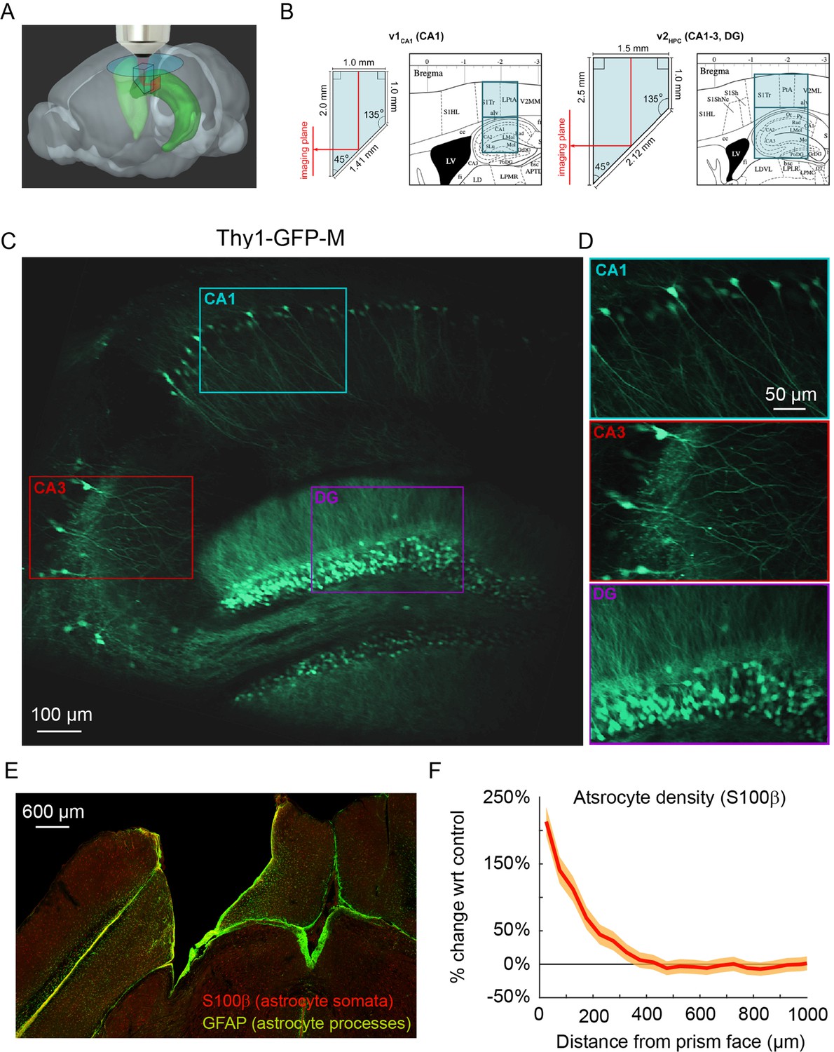
Implanted microperiscopes allow imaging of the hippocampal transverse plane.
(A) Three-dimensional schematic (Wang et al., 2020) illustrating microperiscope implantation and light path for hippocampal imaging. (B) Schematics (Paxinos and Franklin, 2001) showing the imaging plane location of v1CA1 (1 mm imaging plane, 2 mm total length) and v2HPC (1.5 mm imaging plane, 2.5 mm total length) microperiscopes. (C) Tiled average projection of the transverse imaging plane using the v2HPC microperiscope implant in a Thy1-GFP-M transgenic mouse. Scale bar = 100 μm. (D) Enlarged images of hippocampal subfields (CA1, CA3, DG) corresponding to the rectangles in (C). Scale bar = 50 μm. (E) Example histological section stained for astrocyte cell bodies (S100β, red) and processes (GFAP, green). Scale bar = 600 μm. (F) Quantification of astrocyte density as a function of distance from the microperiscope face, normalized to the density in the unimplanted contralateral hemisphere (n=2 mice; 288 and 316 days post-implant; mean ± bootstrapped s.e.m.).
Figure 1—figure supplement 1
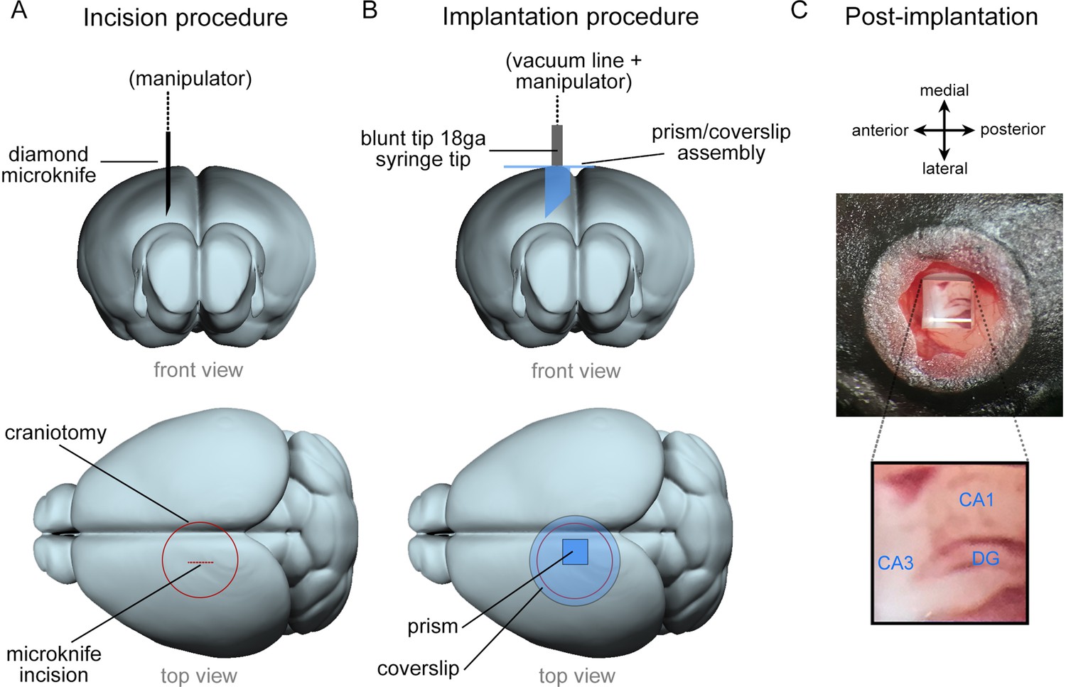
Overview of microperiscope implantation surgery.
(A) Schematic view from front (top row) and top (bottom row) of mouse brain indicating placement of the incision. The incision is made using a diamond microknife prior to the implantation of microperiscope. The microknife bevel faces medial to leave a flat surface for the microperiscope face. (B) Schematic view from front (top row) and top (bottom row) of the brain during microperiscope implantation. The microperiscope is attached to the coverglass prior to implantation using optical glue, and the assembly is lowered into the incision using a blunt 18-gauge syringe mounted on a manipulator and held using a vacuum line. Once the assembly has been cemented to the skull, the vacuum is released, and the manipulator removed. The microperiscope faces lateral for imaging of the transverse plane of the dorsomedial hippocampus. (C) Post-implantation view of microperiscope assembly, with identified hippocampal subregions.
Figure 1—figure supplement 2
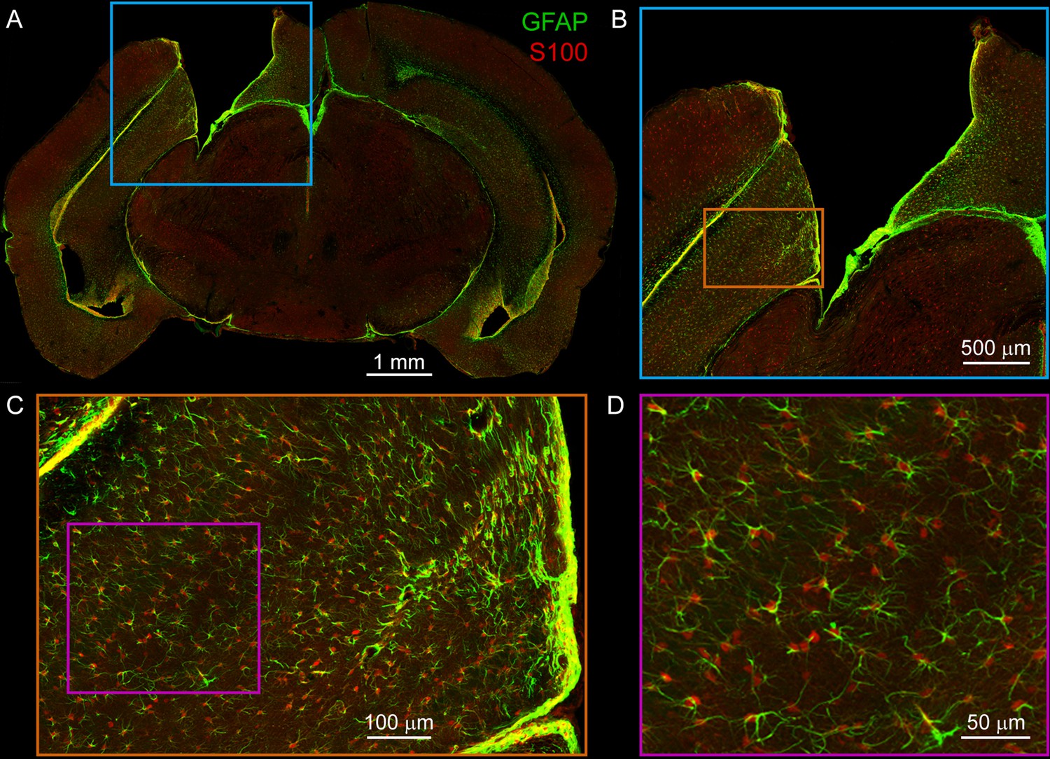
Additional visualization of astrocyte immunohistochemistry.
(A) Mosaic confocal image of entire slice from mouse implanted with v2HPC microperiscope. Note that tissue shrinkage around implant margins increases apparent implant size. Green: GFAP (astrocyte processes); Red: S100β (astrocyte cell bodies); scale bar = 1 mm. (B) Higher zoom image from cyan box in (A). Scale bar = 500 μm. (C) Higher zoom image from orange box in (B). Scale bar = 100 μm. (D) Higher zoom image from cyan box in (C). Note co-staining of individual astrocytes with GFAP and S100β; S100β used for all quantification (Figure 1F) due to improved localization of cell bodies. Scale bar = 50 μm.
Figure 2
Optical characterization of cranial window and microperiscopes.
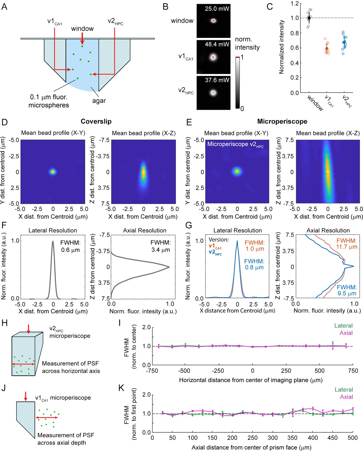
(A) Schematic of signal yield and resolution characterization experiments to allow comparison of microperiscopes (v1CA1 and v2HPC) and standard coverslip window (0.15 mm thickness) using 0.2 m fluorescent microspheres imaged with a 16×/0.8 NA objective. (B) Example microspheres imaged through the window, v1CA1 microperiscope, and v2HPC microperiscope. Laser power was gradually increased to the minimum level necessary to saturate the centroid of the microsphere with all other imaging parameters held constant. (C) Distribution of signal intensity values (n=12 microspheres for each condition), measured as the reciprocal of the minimum laser intensity for saturation, and normalized to the mean intensity through the window (v1CA1: 59.0% ± 6.6%; v2HPC: 67.2% ± 8.5%, mean ± s.d.). (D) Average X-Y profile (left) and X-Z profile (right) of fluorescent microspheres (n=58 microspheres) imaged through the window. (E) Average X-Y profile (left) and X-Z profile (right) of fluorescent microspheres (n=48 microspheres) imaged through the v2HPC microperiscope (2.5 mm path length through glass). (F) Plot of normalized fluorescence intensity profile of X dimension (lateral resolution; FWHM = 0.6 μm) and Z dimension (axial resolution; FWHM = 3.4 m) through the centroid of the microsphere (n=58 microspheres) imaged through the window. (G) Plot of normalized fluorescence intensity profile of X dimension (lateral resolution; v1CA1 FWHM = 1.0 m, orange; v2HPC FWHM = 0.8 m, blue) and Z dimension (axial resolution; v1CA1 FWHM = 11.7 m; v2HPC FWHM = 9.5 m) through the centroid of the microsphere (n=28 microspheres for v1CA1, n=48 microspheres for v2HPC). (H) Schematic of the experiment used to characterize lateral and axial resolution across the horizontal axis of the microperiscope. Version v2HPC used for larger horizontal range. (I) Lateral (green) and axial (magenta) FWHM (mean ± s.e.m.) of average microsphere profile as a function of horizontal distance from the center of the microperiscope. FWHM values normalized to the mean at the center of the imaging axis (–100 to +100 m). There was no effect of horizontal position on lateral FWHM (F(14, 593)=0.53, p=0.91) or axial FWHM (F(14, 593)=0.91, p=0.55; one-way ANOVA). (J) Schematic of the experiment used to measure resolution as a function of distance from the microperiscope face. Version v1CA1 used for larger working distance. (K) Lateral (green) and axial (magenta) FWHM (mean ± s.e.m.) of average microsphere profile as a function of distance from the face of the microperiscope, with FWHM values normalized to the closest position (25 m). There was no effect of distance of imaging depth on lateral FWHM (F(19, 109)=0.53, p=0.26). There was a difference for axial FWHM (F(19, 109)=2.51, p=0.002; one-way ANOVA), though no individual position was significantly different from the first position when corrected for multiple comparisons (Tukey-Kramer post hoc test).
Figure 3 with 2 supplements
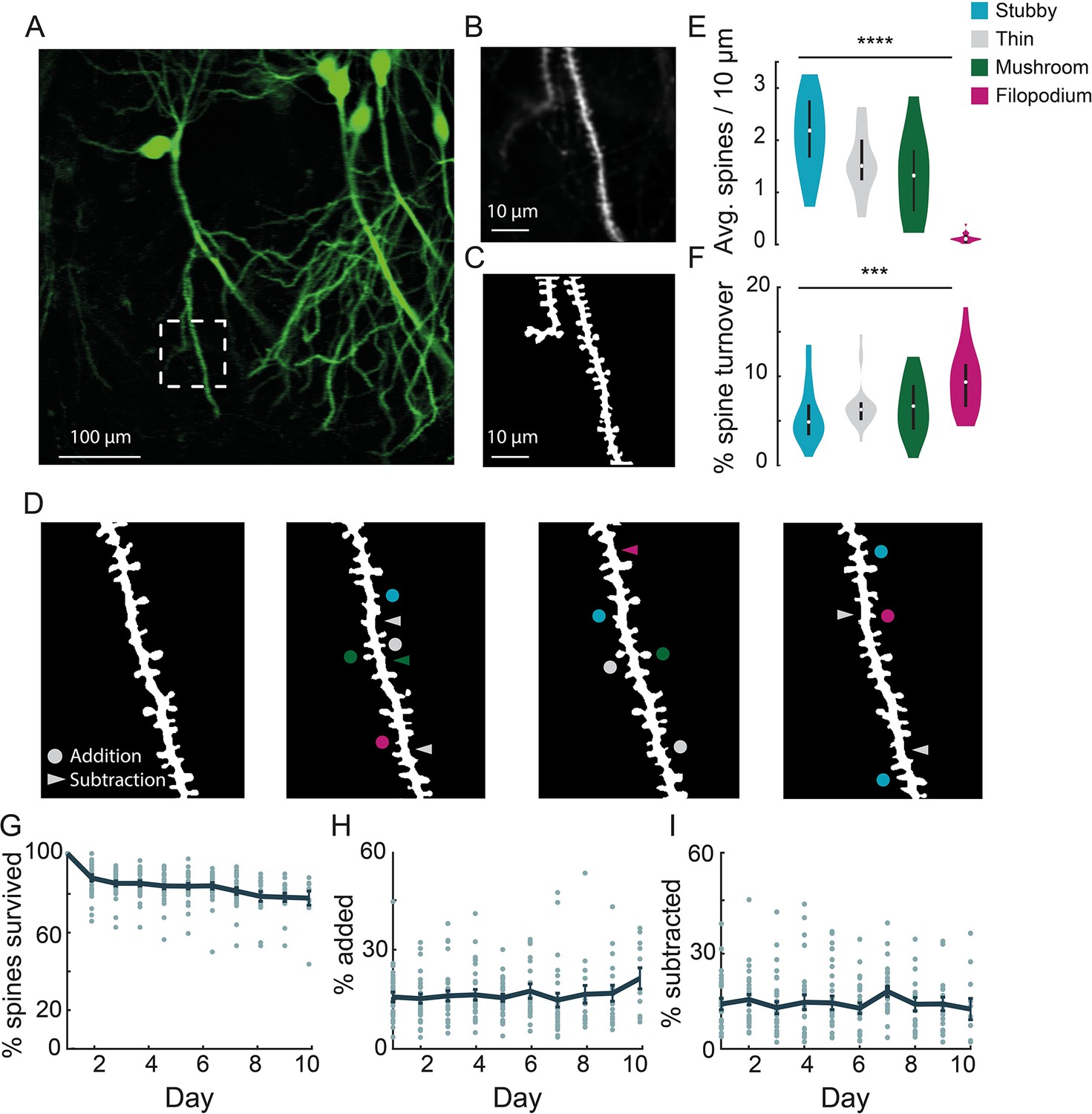
Chronic imaging of spine morphology in CA1 apical dendrites.
(A) Average projection of CA1 neurons sparsely expressing a GFP reporter (Thy1-GFP-M) imaged through the v1CA1 microperiscope. Scale bar = 100 μm. (B) Weighted projection (see Materials and methods) of the apical dendrites shown in the dashed box of (A). Scale bar = 10 μm. (C) Filtered and binarized image (Figure 3—figure supplement 1A; see Materials and methods) of the dendrites in (B) to allow for the identification and classification of individual dendritic spines. Scale bar = 10 μm. (D) Tracking CA1 dendritic spines over consecutive days on a single apical dendrite. Arrowheads indicate subtracted spines and circles indicate added spines. Colors indicate spine type of added and subtracted spines: filopodium (magenta), thin (gray), stubby (blue), and mushroom (green). (E) Average number of spines per 10 μm section of dendrite, for each of the four classes of spine (n=26 dendrites from 7 mice); one-way ANOVA, F(3,100) = 51.47, ****p<0.0001. Error bars indicate the interquartile range (75th percentile minus 25th percentile) and circle is median. (F) Percent spine turnover across days in each spine type (n=26 dendrites from 7 mice); one-way ANOVA, F(3,100) = 7.17, ***p<0.001. Error bars indicate the interquartile range (75th percentile minus 25th percentile) and circle is median. (G) Spine survival fraction across processes (n=26 dendrites from 7 mice) recorded over 10 consecutive days. (H) Percent of spines added between days over 10 days of consecutive imaging. (I) Percent of spines subtracted between days over 10 days of consecutive imaging.
Figure 3—figure supplement 1
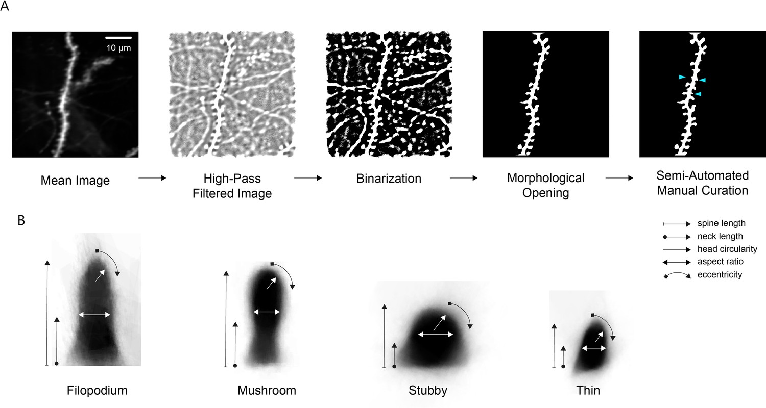
Dendritic morphology image processing pipeline and spine classification.
(A) Steps in dendritic morphology image processing pipeline (see Materials and methods). Weighted mean image is obtained by acquiring average projections from four planes spaced by 3 μm and weighting the images around the brightest part of the dendrite. Next, the mean image is high-pass filtered to reveal fine structures. The image is then binarized using a global threshold, to filter out less prominent dendrites. Morphological opening is applied to remove any elements of the high-pass filtered image that survive the binarization process that are too small to be the principal dendrite. A semi-automated manual curation process is then used to add back any individual spines that were lost during binarization and remove any unwanted dendritic segments. Cyan arrowheads indicate manually added spines. To isolate the spines, the image is skeletonized and structures that protrude laterally from the dendritic shaft and have a total area of >1 μm2 are identified as spines. Scale bar = 10 μm. (B) Mean profile of all filopodium, mushroom, stubby, and thin spines (n=47, 431, 695, and 495, respectively), computed by averaging across the registered spines of each morphological classification. Spines were classified according to spine length, neck length, neck width, head circularity, and eccentricity (see Materials and methods).
Figure 3—figure supplement 2
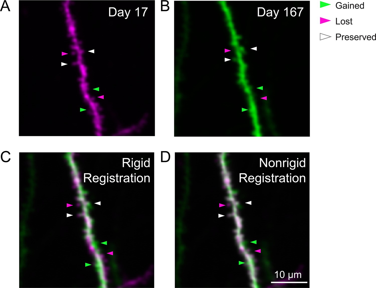
Long-term imaging of the same dendrite.
(A) Example weighted average projection of a dendritic process imaged 17 days after microperiscope implantation. (B) Same as (A), imaged 167 days after microperiscope implantation (150 days later). Arrowheads mark examples of spines that are present in locations along the dendrite at day 17, but not day 167 (‘lost’, magenta), present in locations at day 167, but not 17 (‘gained’, green), and present in locations at both days 17 and 167 (‘preserved’, white). Note that the dendrite was not imaged continuously, so we cannot be certain the preserved spines were there during the entire duration. (C) Images from (A) and (B) overlaid, using rigid registration. (D) Images from (A) and (B) overlaid, using non-rigid registration (see Materials and methods). Scale bar = 10 μm.
Figure 4 with 2 supplements
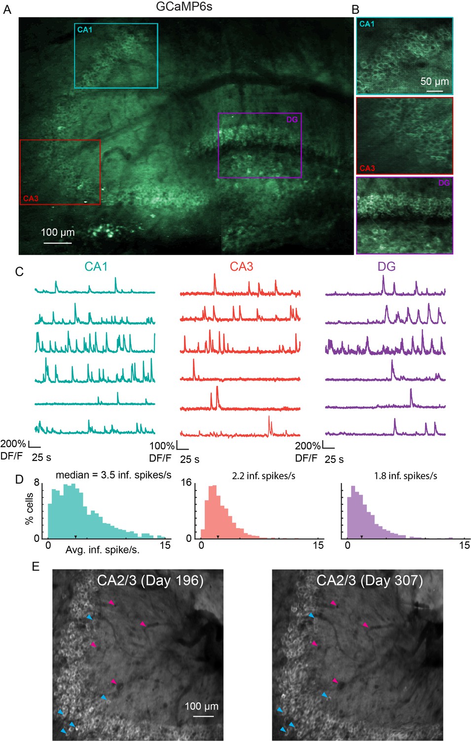
Microperiscope imaging of calcium dynamics across subfields in awake mice.
(A) Example tiled image (as in Figure 1C) for a single panexcitatory transgenic GCaMP6s mouse (Slc17a7-GCaMP6s). Scale bar = 100 μm. (B) Enlarged images of each hippocampal subfield (CA1, CA3, DG) corresponding to the rectangles in (A). Scale bar = 50 μm. (C) Example GCaMP6s normalized fluorescence time courses (% DF/F) for identified cells in each subfield. (D) Distribution of average inferred spiking rate during running for each hippocampal subfield (CA1, CA3, DG; see Materials and methods). Median is marked by black arrowhead. (E) Example average projection of CA2/3 imaging plane 196 days post implantation (left) and 111 days later. Image was aligned using non-rigid registration (see Materials and methods) to account for small tissue movements. Magenta arrowheads mark example vasculature and blue arrowheads mark example neurons that are visible in both images. Scale bar = 100 μm.
Figure 4—figure supplement 1

Simultaneous imaging of all three hippocampal subfields.
Maximum projection, and example GCaMP6s fluorescence time courses for identified cells, from a recording in which CA1 (n=55 cells), CA3 (n=158), and DG (n=28) were simultaneously recorded from the same image plane. Scale bar = 100 μm.
Figure 4—figure supplement 2
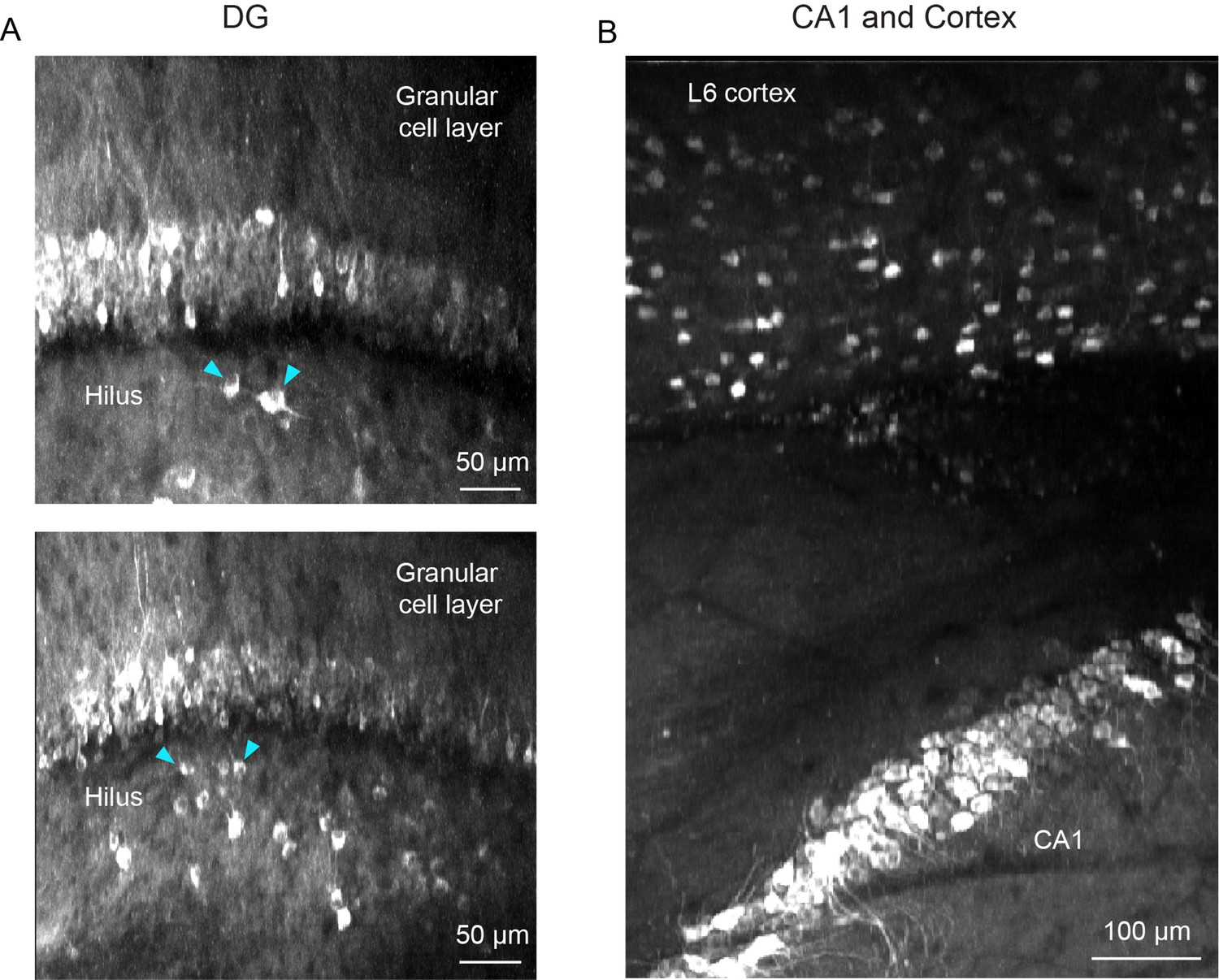
Additional applications for microperiscope imaging.
(A) Two maximum projections of imaging planes in which both the granular cell layer and the hilus in the dentate gyrus (DG) could be imaged simultaneously. Example putative mossy cells indicated with cyan arrowheads. Scale bar = 50 μm. (B) Maximum projection from an imaging session in which both CA1 and L6 of the neocortex are visible, allowing simultaneous imaging of neurons in CA1 and deep layers of the parietal cortex. Scale bar = 100 μm.
Figure 5 with 1 supplement
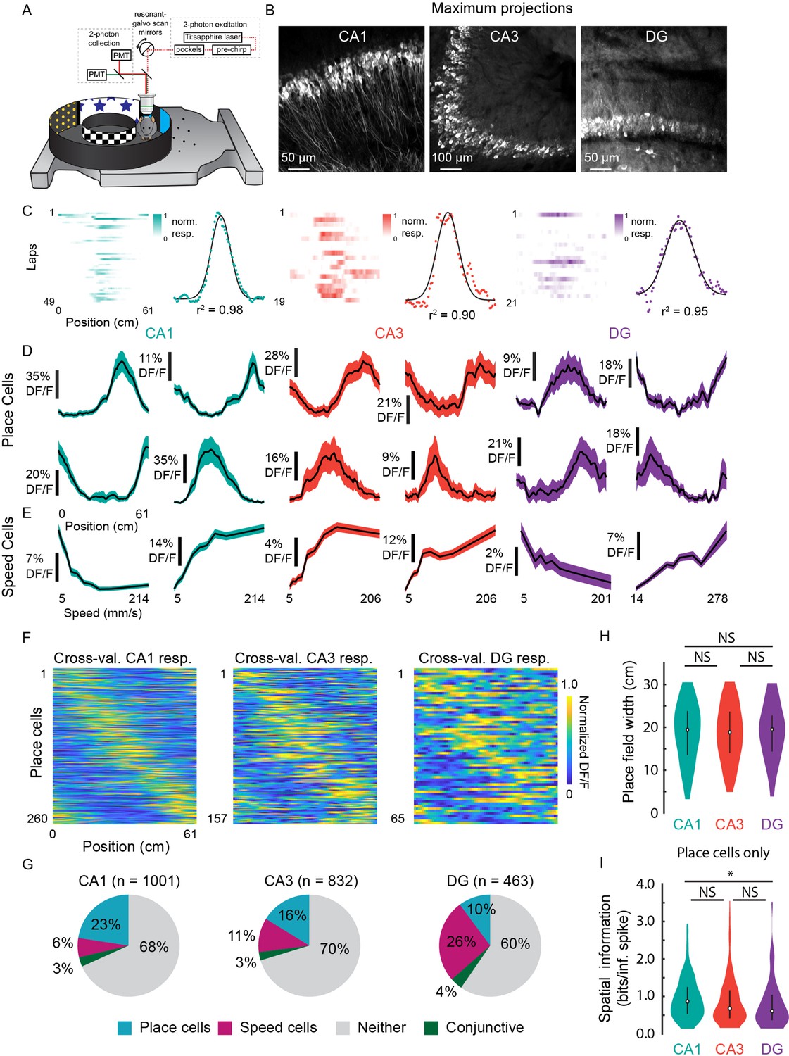
Prevalence of place (PCs) and speed cells (SCs) across hippocampal subfields.
(A) Schematic of air-lifted carbon fiber circular track (250 mm outer diameter) that the mice explored during imaging (Video 4). Four sections of matched visual cues lined the inner and outer walls. (B) Example maximum projections of GCaMP6s-expressing neurons in each subfield. Scale bar = 50, 100, 50 μm, respectively. (C) Lap-by-lap activity and Gaussian fits, with r2 value reported, of example PCs for each hippocampal subregion to illustrate our process of identifying PCs (see Materials and methods). (D) Examples of mean normalized calcium response (% DF/F) vs. position along the circular track for four identified PCs in each subregion. Shaded area is s.e.m. (E) Examples of mean calcium response (% DF/F) vs. speed along the circular track for two identified SCs in each subregion. Shaded area is s.e.m. (F) Cross-validated average responses (normalized % DF/F) of all PCs found in each subfield, sorted by the location of their maximum activity. Responses are plotted for even trials based on peak position determined on odd trials to avoid spurious alignment. (G) Distribution of cells that were identified as PCs, SCs, conjunctive PC + SCs, and non-coding in each subregion. (H) Distribution of place field width for all PCs in each subregion. Error bars indicate the interquartile range (75th percentile minus 25th percentile) and circle is median. Two-sample Kolmogorov-Smirnov test: CA1-CA3, p=0.67; CA3-DG, p=0.70; CA1-DG, p=0.51. NS, not significant (p>0.05). (I) Distribution of spatial information (bits per inferred spike) for all PCs in each subregion. Error bars and circle are the same as in (H). Two-sample Kolmogorov-Smirnov test: CA1-CA3, p=0.05; CA3-DG, p=0.36; CA1-DG, p=0.01. *p<0.05.
Figure 5—figure supplement 1
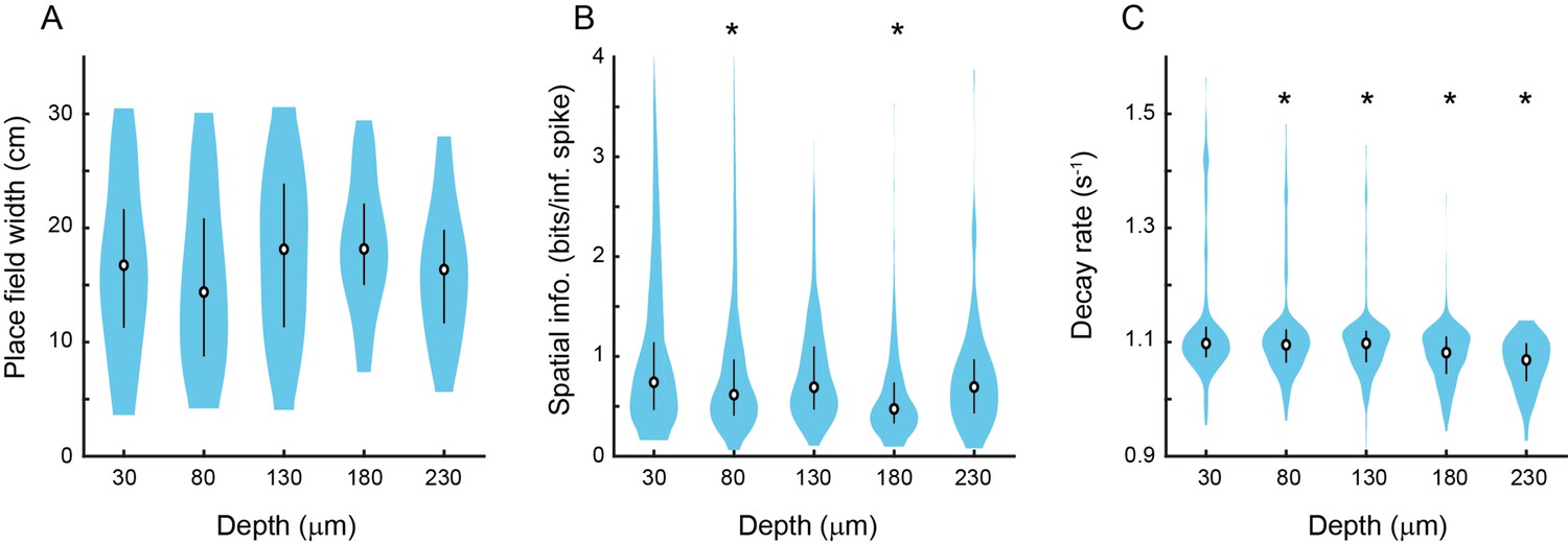
Place cell properties as a function of distance from the face of the microperiscope.
(A) Place field width as a function of imaging depth relative to the microperiscope face. Error bars indicate the interquartile range (75th percentile minus 25th percentile) and circle is median (F(4, 241)=1.6, p=0.17, one-way ANOVA). (B) Same as (A), but for spatial information of place cells (F(4, 1872)=15.9, p=8.6 × 10⁻¹³, one-way ANOVA; Tukey-Kramer post hoc test for depth vs. 30 μm: 80 μm, p=1.1 × 10⁻³; 130 μm, p=0.34; 180 μm, p=9.92 × 10⁻⁹; 230 μm, p=0.15). *p<0.05 Tukey-Kramer post hoc test. (C) Same as (A), but for decay rate (Friedrich et al., 2017) of place cells (F(4, 1872)=29.8, p=4.5 × 10⁻²⁴; Tukey-Kramer post hoc test for depth vs. 30 μm: 80 μm, p=6.70 × 10⁻³; 130 μm, p=9.38 × 10⁻⁷; 180 μm, p=9.92 × 10⁻⁹; 230 μm, p = 9.92 × 10⁻⁹). *p<0.05 Tukey-Kramer post hoc test.
Figure 6 with 1 supplement
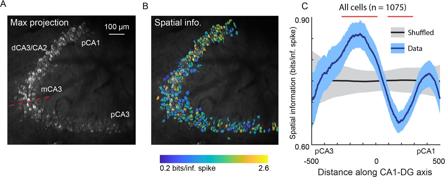
Spatial information of neurons varies along the DG-to-CA1 axis.
(A) Maximum projection of an example DG-to-CA1 axis recording. Approximate locations of CA3 and CA1 subfields are labeled. Inflection point labeled with red line. Scale bar = 100 μm. (B) Spatial information (bits/inferred spike), pseudo-colored on a logarithmic scale, for each neuron, overlaid on the maximum projection in (A). (C) Spatial information, as a function of distance along the DG-to-CA1 axis (pCA3 to dCA1), calculated with a sliding window; mean ± bootstrapped s.e.m.; real data (blue), shuffled control (black). Red lines indicate values that are outside the shuffled distribution (p<0.05). A general linear F-test against a flat distribution with the same mean revealed significant non-uniformity: F(4, 1047)=5.10, p=4.6 × 10⁻⁴ (cells with distance greater than 600 or less than –600 were not included in the statistical analysis).
Figure 6—figure supplement 1
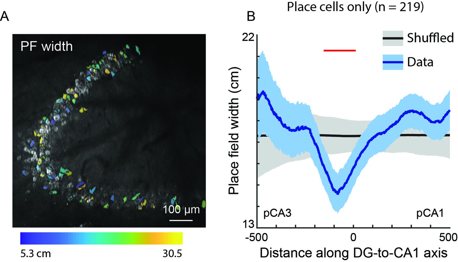
Place field width does not significantly vary along the DG-to-CA1 axis.
(A) Place field width, pseudo-colored for each place cell, overlaid on the maximum projection from Figure 6A. Any cell that was not a place cell is not pseudo-colored. Scale bar = 100 μm. (B) Place field width, as a function of distance along the DG-to-CA1 axis (pCA3 to pCA1), of real data (blue) vs. shuffled control (black). Shaded area is s.e.m. Red line indicates individual positions with place field values that were outside of the shuffled distribution (p<0.05). A general linear F-test, against a flat distribution with the same mean, revealed no significant non-uniformity: F(4, 206)=1.63, p=0.17 (cells with distance greater than 600 or less than –600 were not included in the statistical analysis).
Author response image 1
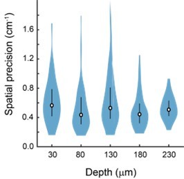
Spatial precision does not vary significantly with depth of imaging plane from the face of the periscope.
Videos
Video 1
Demonstration of two-photon imaging of an Slc17a7-GCaMP6s mouse through the microperiscope.
Recording starts in the superficial cortex in front of microperiscope, then moves through the microperiscope to the hippocampus, zooming in on subfields CA1, CA3, and DG.
Video 2
Calcium activity in subfield CA1 in an Slc17a7-GCaMP6s mouse imaged through the microperiscope.
Video 3
Calcium activity in subfield DG in an Slc17a7-GCaMP6s mouse imaged through the microperiscope.
Video 4
Mouse running in the floating chamber circular track.
Ambient light is higher than usual levels for improved video quality.
Additional files
Download links
A two-part list of links to download the article, or parts of the article, in various formats.
Downloads (link to download the article as PDF)
Open citations (links to open the citations from this article in various online reference manager services)
Cite this article (links to download the citations from this article in formats compatible with various reference manager tools)
Long-term transverse imaging of the hippocampus with glass microperiscopes
eLife 11:e75391.
https://doi.org/10.7554/eLife.75391


