Neuronal origins of reduced accuracy and biases in economic choices under sequential offers
- Department of Neuroscience, Washington University in St. Louis, United States
- Department of Economics, Washington University in St. Louis, United States
- Department of Biomedical Engineering, Washington University in St. Louis, United States
Figures
Figure 1

Computational framework.
Information about sensory input, stored memory, and the motivational state is integrated during the computation of offer values. In orbitofrontal cortex (OFC), offer value cells provide the primary input to a decision circuit composed of chosen juice cells and chosen value cells. The detailed structure of the decision circuit is not well understood, but previous work indicates that decisions under sequential offers rely on circuit inhibition. In essence, neurons encoding the value of the first offer (offer1) indirectly impose a negative offset on the activity of chosen juice cells associated with the second offer (offer2). Notably, this circuit might also subserve working memory. The decision output, captured by the activity of chosen juice cells, informs other brain regions that transform it into a suitable action plan. Choice measured behaviorally is ultimately defined by the motor response. This framework highlights the fact that choice biases and/or noise might emerge at multiple computational stages. The arrows indicated here capture only the primary connections.
Figure 2
Experimental design and choice biases.
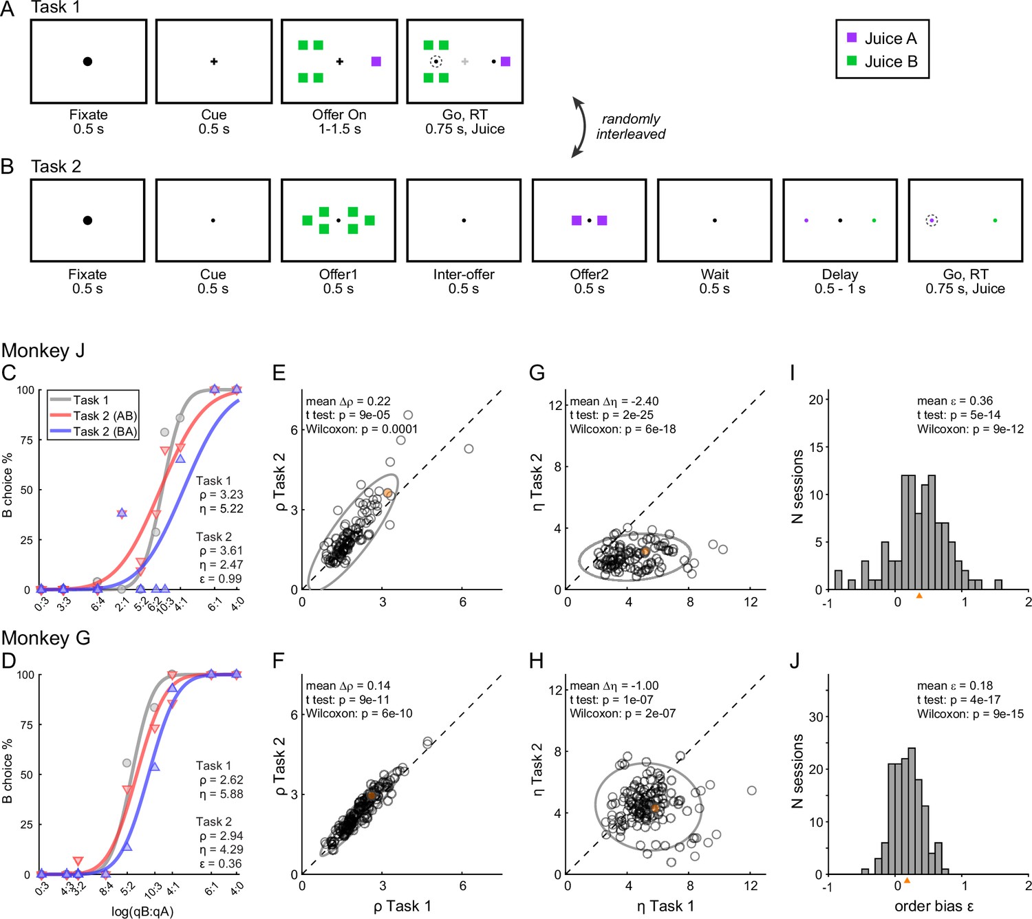
(A, B) Experimental design. Animals chose between two juices offered in variable amounts. Offers were represented by sets of color squares. For each offer, the color indicated the juice type and the number of squares indicated the juice amount. In each session, trials with Tasks 1 and 2 were randomly interleaved. In Task 1, two offers appeared simultaneously on the left and right sides of the fixation point. In Task 2, offers were presented sequentially, spaced by an interoffer delay. After a wait period, two saccade targets matching the colors of the offers appeared on the two sides of the fixation point. The left/right configuration in Task 1, the presentation order in Task 2, and the left/right position of the saccade targets in Task 2 varied randomly from trial to trial. In any session, the same set of offer types was used for both tasks. (C) Example session 1. The percent of B choices (y-axis) is plotted against the log quantity ratio (x-axis). Each data point indicates one offer type in Task 1 (gray circles) or Task 2 (red and blue triangles for AB trials and BA trials, respectively). Sigmoids were obtained from probit regressions. The relative value (ρ) and sigmoid steepness (η) measured in each task and the order bias (ε) measured in Task 2 are indicated. In this session, the animal presented all three biases. Compared to Task 1, choices in Task 2 were less accurate (ηTask2 < ηTask1) and biased in favor of juice A (ρTask2 > ρTask1; preference bias). Furthermore, choices in Task 2 were biased in favor of offer2 (ε > 0; order bias). (D) Example session 2. Same format as panel C. (E, F) Comparing relative value across choice tasks. Each data point represents one session and gray ellipses indicate 90% confidence intervals. For both monkeys, relative values in Task 2 (y-axis) were significantly higher than in Task 1 (x-axis). Furthermore, the main axis of each ellipse was rotated counterclockwise compared to the identity line. (G, H) Comparing the sigmoid steepness across choice tasks. For both monkeys, sigmoids were consistently shallower (smaller η) in Task 2 compared to Task 1. (I, J) Order bias, distribution across sessions. Both monkeys presented a consistent bias favoring offer2 (mean(ε) > 0). Panels C, E, G, and I are from monkey J (N = 101 sessions); panels D, F, H, and J are from monkey G (N = 140 sessions). Sessions shown in panels C and D are highlighted in yellow in panels E, F, G, and H. Triangles in panels I and J indicate the mean. Statistical tests and exact p values are indicated in each panel.
Figure 3
Order bias and preference bias.
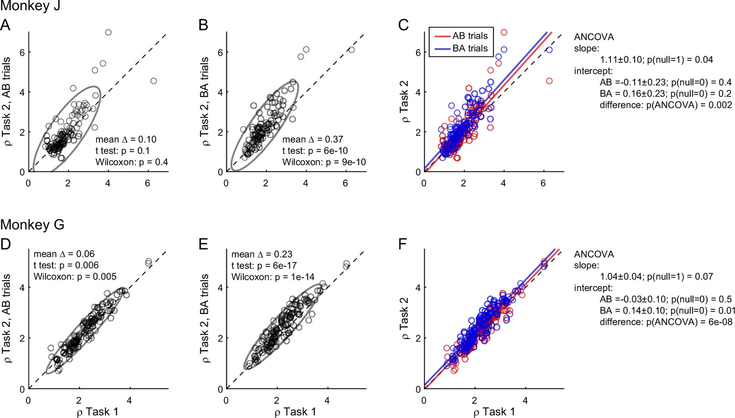
(A–C) Monkey J (N = 101 sessions). In panels A and B, ρTask2,AB and ρTask2,BA (y-axis) are plotted against ρTask1 (x-axis). Each data point represents one session and gray ellipses indicate 90% confidence intervals. The main axis of both ellipses is rotated counterclockwise compared to the identity line (preference bias). In addition, the ellipse in panel B is displaced upwards compared to that in panel A (order bias). In panel C, the same data are pooled and color coded. The two lines are from an ANCOVA (covariate: order; parallel lines). The regression slope is significantly >1 (preference bias) and the two intercepts differ significantly from each other (order bias). (D–F) Monkey G (N = 140 sessions). Same format. The results closely resemble those for monkey J but the preference bias is weaker.
Figure 4 with 1 supplement
Lower choice accuracy in Task 2 reflects weaker offer value signals.
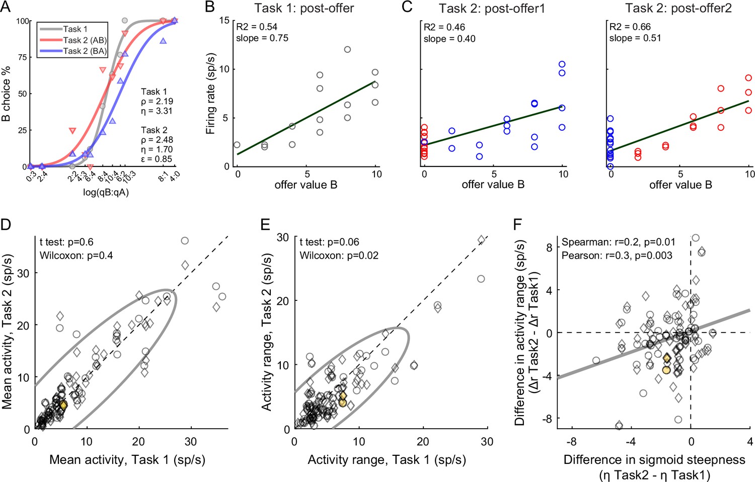
(A–C) Weaker offer value signals in Task 2, example cell. Panel A illustrates the choice pattern. Panel B illustrates the neuronal response measured in Task 1 (post-offer time window). Each data point represents one trial type. In C, two panels illustrate the neuronal responses measured in Task 2 (post-offer1 and post-offer2 time windows). Each data point represents one trial type; red and blue colors are for AB and BA trials, respectively. In panels B and C, firing rates (y-axis) are plotted against variable offer value B and gray lines are from linear regressions. Notably, the cell has lower activity range in Task 2 than in Task 1. (D, E) Weaker offer value signals in Task 2, population analysis (N = 109 offer value cells). The two panels illustrate the results for the mean activity and the activity range, respectively. In each panel, x- and y-axis represent measures obtained in Task 1 and Task 2, respectively. Each data point represents one cell. For each cell, we examined one time window (post-offer) in Task 1 and two time windows (post-offer1 and post-offer2) in Task 2. Circles and diamonds refer to post-offer1 and post-offer2 time windows, respectively. Measures of mean activity measured in the two tasks (panel D) were statistically indistinguishable. In contrast, activity ranges (panel E) were significantly reduced in Task 2 compared to Task 1. Statistical tests and exact p values are indicated in each panel. The example cell shown in panels A–C is highlighted in orange in panels D and E. (F) Offer value signals and choice accuracy (N = 109 cells). For each offer value cell, we computed the activity range Δr in each task (see Methods). Here, the difference in activity range Δr = ΔrTask2 − ΔrTask1 (y-axis) is plotted against the difference in sigmoid steepness Δη = ηTask2 − ηTask1 measured in the same session (x-axis). The two measures were significantly correlated across the population. The gray line in panel F is from a linear regression. This analysis was restricted to 53 cells significantly tuned in the post-offer time window (Task 1) and post-offer1 time window (Task 2), and 56 cells significantly tuned in the post-offer time window (Task 1) and post-offer2 time window (Task 2).
Figure 4—figure supplement 1
Comparing tuning functions across choice tasks.
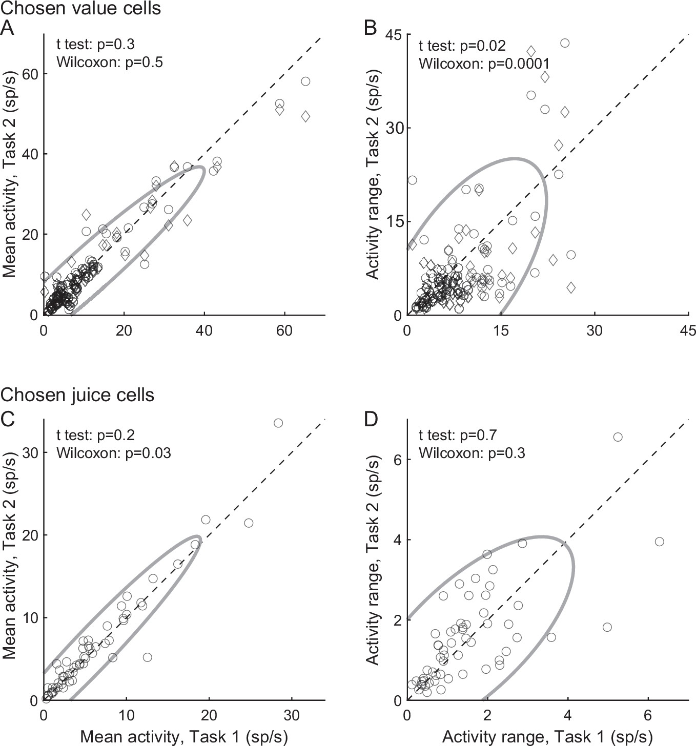
(A, B) Chosen value cells (N = 104). Same format as in Figure 4A, B. For each cell, we examined one time window (post-offer) in Task 1 and two time windows (post-offer1 and post-offer2) in Task 2. Both the mean activity and the activity range were statistically indistinguishable across tasks. (C, D) Chosen juice cells (N = 58). For each cell, we examined the same time window (post-juice) in both tasks. Both the mean activity and the activity range were statistically indistinguishable across choice tasks. In panels B–D, legends report the results of statistical tests. For both cell groups, fluctuations in activity range were not correlated with fluctuations in choice variability across the population (in both analyses, |r| < 0.1, p > 0.4; not shown). Only cells presenting significant tuning in the relevant time windows were included in each panel (see Methods).
Figure 5 with 1 supplement
Fluctuations in order bias and fluctuations in the activity of chosen value cells.
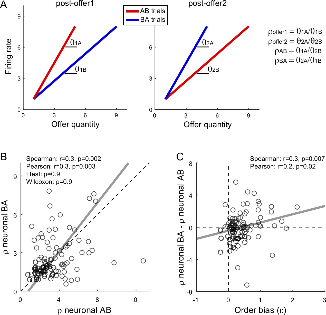
(A) Neuronal measures of relative value. The two panels represent in cartoon format the response of a chosen value cell in the post-offer1 and post-offer2 time window (Task 2). In each of these time windows, chosen value cells encode the value of the offer on display. Here, the two axes correspond to the firing rate (y-axis) and to the offered juice quantity (x-axis). The two colors correspond to the two orders (AB, BA). In each time window, two linear regressions provide two slopes, proportional to the value of the two juices. From the four measures θ1A (left panel, red), θ1B (left panel, blue), θ2A (right panel, blue), and θ2B (right panel, red), we derive four neuronal measures of relative value (Methods, Equations 13–16). (B) Neuronal measures of relative value in AB trials and BA trials (N = 96 cells). The x- and y-axis correspond to ρneuronalAB and ρneuronalBA, respectively. Each data point represents one cell. The two measures are strongly correlated. The gray line is from a Deming regression. (C) Fluctuations of relative value and fluctuations in order bias (N = 96 cells). For each chosen value cell, we quantified the difference in the neuronal measure of relative value Δρneuronal = ρneuronalAB − ρneuronalBA. Here, the x-axis is the order bias (ε), the y-axis is Δρneuronal, and each data point corresponds to one cell. The gray line is from a linear regression. Statistical tests and exact p values are indicated in each panel. This analysis was restricted to 96 cells that had significant θ1A, θ1B, θ2A, and θ2B. Fluctuations of Δρneuronal correlated with fluctuations of ε across the population. Of note, the regression line has a negative intercept and the data cloud seems displaced downwards compared to what one might expect. As a result, Δρneuronal was on average close to 0. We cannot provide a clear interpretation for this observation and future work shall revisit this issue.
Figure 5—figure supplement 1
The order bias does not reflect differences in the tuning of offer value cells.
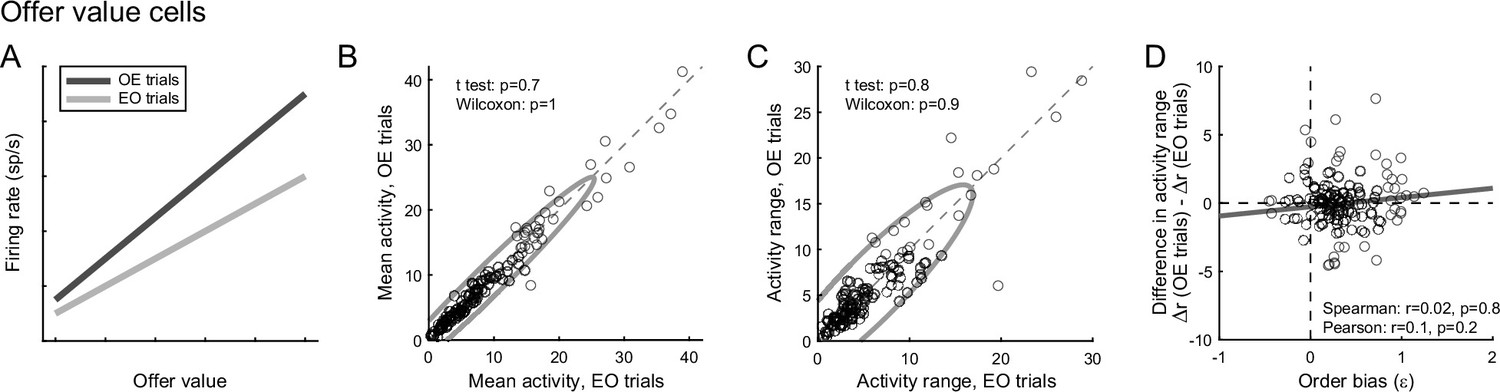
(A) Rationale for the analysis. The two lines represent in cartoon format the hypothetical tuning functions of an offer value cell in the post-offer1 time window (EO trials) and in the post-offer2 time window (OE trials). The order bias would be explained if offer value cells encoded, other things equal, higher values in OE trials than in EO trials. This would be the case if the mean activity and/or the activity range were higher in OE trials, as depicted here. (B) Comparison of mean activity. x- and y-axis represent the mean activity measured in post-offer1 (EO trials) and post-offer2 (OE trials) time windows, respectively. Each data point represents one cell. The two measures were statistically indistinguishable across the population. (C) Comparison of activity range. Same format as panel B. The two measures were statistically indistinguishable across the population. (D) Lack of correlation between differences in activity range and order bias. Across the population, we did not find any correlation between the difference in activity range (y-axis) and the order bias. Exact p values are indicated in each panel. For this figure, we pooled neurons associated with A and B, and neurons with positive and negative encoding (N = 128 cells total). This analysis was restricted to cells significantly tuned in post-offer1 and post-offer2 time windows (Task 2). An additional 11 cells were removed because measures of order bias were detected as outliers by the interquartile criterion (see Methods). Including these cells in the analysis did not substantially alter the results. A similar analysis conducted on chosen value cells yielded similar negative results (not shown).
Figure 6
Order bias and circuit inhibition.
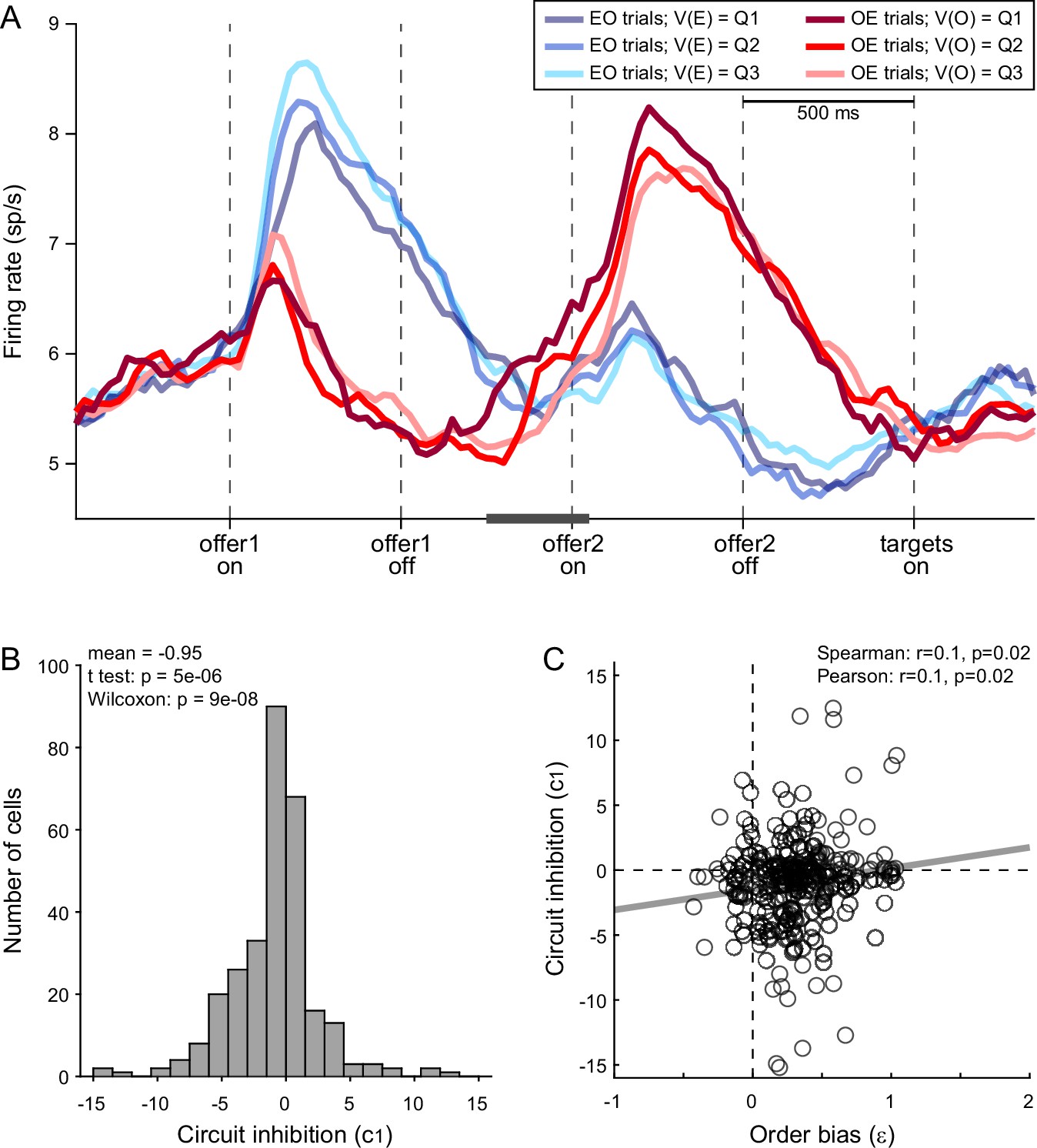
(A) Circuit inhibition in chosen juice cells (primary data set, N = 160 cells). For each chosen juice cell E and O indicated the encoded juice and the other juice, respectively. We separated EO and OE trials, and divided each group of trials in tertiles based on the value of offer1. For EO trials, this corresponded to V(E); for OE trials, it corresponded to V(O). In this panel, Q1, Q2, and Q3 indicate low, medium, and high values of offer1. In OE trials, shortly before offer2, the activity of chosen juice cells was negatively correlated with V(O) – a phenomenon termed circuit inhibition. For a quantitative analysis of circuit inhibition, we focused on 300ms time window starting 250 ms before offer2 onset (black line). (B) Circuit inhibition for individual cells (N = 295 cells). For each chosen juice cell, we regressed the firing rate against the normalized V(O) (see Methods). The histogram illustrates the distribution of regression slopes (c1), which quantify circuit inhibition for individual cells. The effect was statistically significant across the population (mean = −0.95). (C) Correlation between order bias and circuit inhibition (N = 295 cells). Here, the x-axis is the order bias (ε), the y-axis is circuit inhibition (regression slope c1) and each data point represents one cell. The two measures were significantly correlated across the population. Panel A includes only the primary data set; thus circuit inhibition shown here replicates previous findings (Ballesta and Padoa-Schioppa, 2019). Panels B and C include both the primary and the additional data sets (see Methods). In panels B and C, 47 cells were excluded from the analysis because measures of order bias (ε) or circuit inhibition (c1) were detected as outliers by the interquartile criterion. Including these cells in the analysis did not substantially alter the results. Statistical tests and exact p values are indicated in panels B and C.
Figure 7 with 1 supplement
The preference bias does not reflect differences in the activity of chosen value cells.
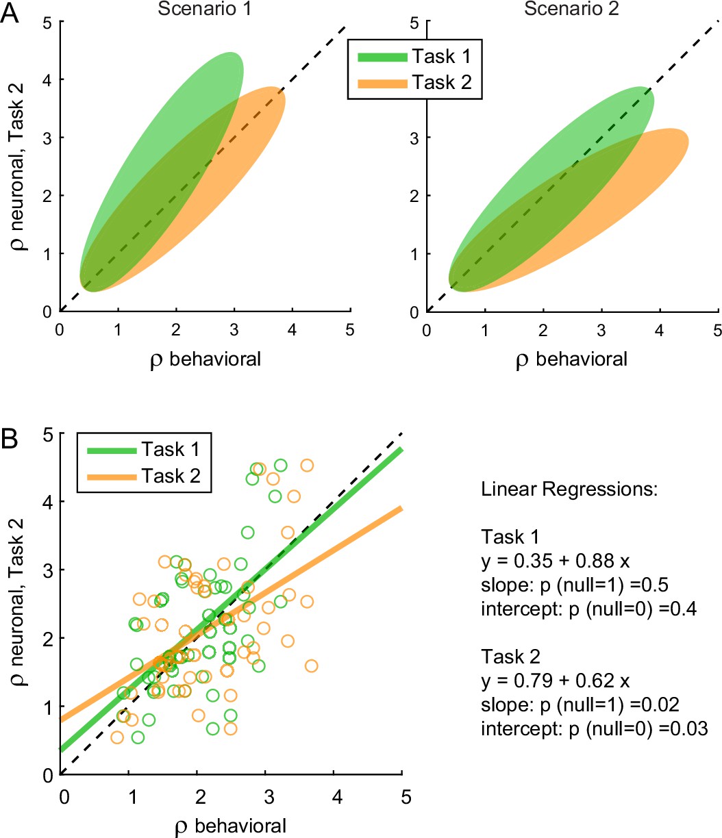
(A) Hypothetical scenarios. The two panels represent in cartoon format two possible scenarios envisioned at the outset of this analysis. In both panels, the x-axis represents behavioral measures from either Task 1 (green) or Task 2 (yellow); the y-axis represents the neuronal measure from Task 2. In scenario 1, the animal assigned higher relative value to juice A in Task 2. Thus, neuronal measures of relative value derived from the activity of chosen value cells in Task 2 (ρneuronalTask2) would align with behavioral measures from the same task (ρbehavioralTask2) and be systematically higher than behavioral measures from Task 1 (ρbehavioralTask1). In scenario 2, the animal assigned the same relative values to the juices in both tasks. Thus, neuronal measures of relative value in Task 2 (ρneuronalTask2) would be systematically lower than behavioral measures from the same task (ρbehavioralTask2) and would align with behavioral measures from Task 1 (ρbehavioralTask1). (B) Empirical results (N = 52 cells). Neuronal measures derived from Task 2 (ρneuronalTask2) are plotted against behavioral measures obtained in Task 1 (ρbehavioralTask1, green) or Task 2 (ρbehavioralTask2), yellow. Lines are from linear regressions. In essence, ρneuronalTask2 was statistically indistinguishable from ρbehavioralTask1 and systematically lower than ρbehavioralTask2. Details on the statistics and exact p values are indicated in the figure. The analysis was restricted to 52 cells that had significant θ1A, θ1B, θ2A, and θ2B. For this analysis, ρneuronalTask2 was taken as equal to ρneuronaloffer2 (Equation 14). Other definitions provided similar results (data not shown).
Figure 7—figure supplement 1
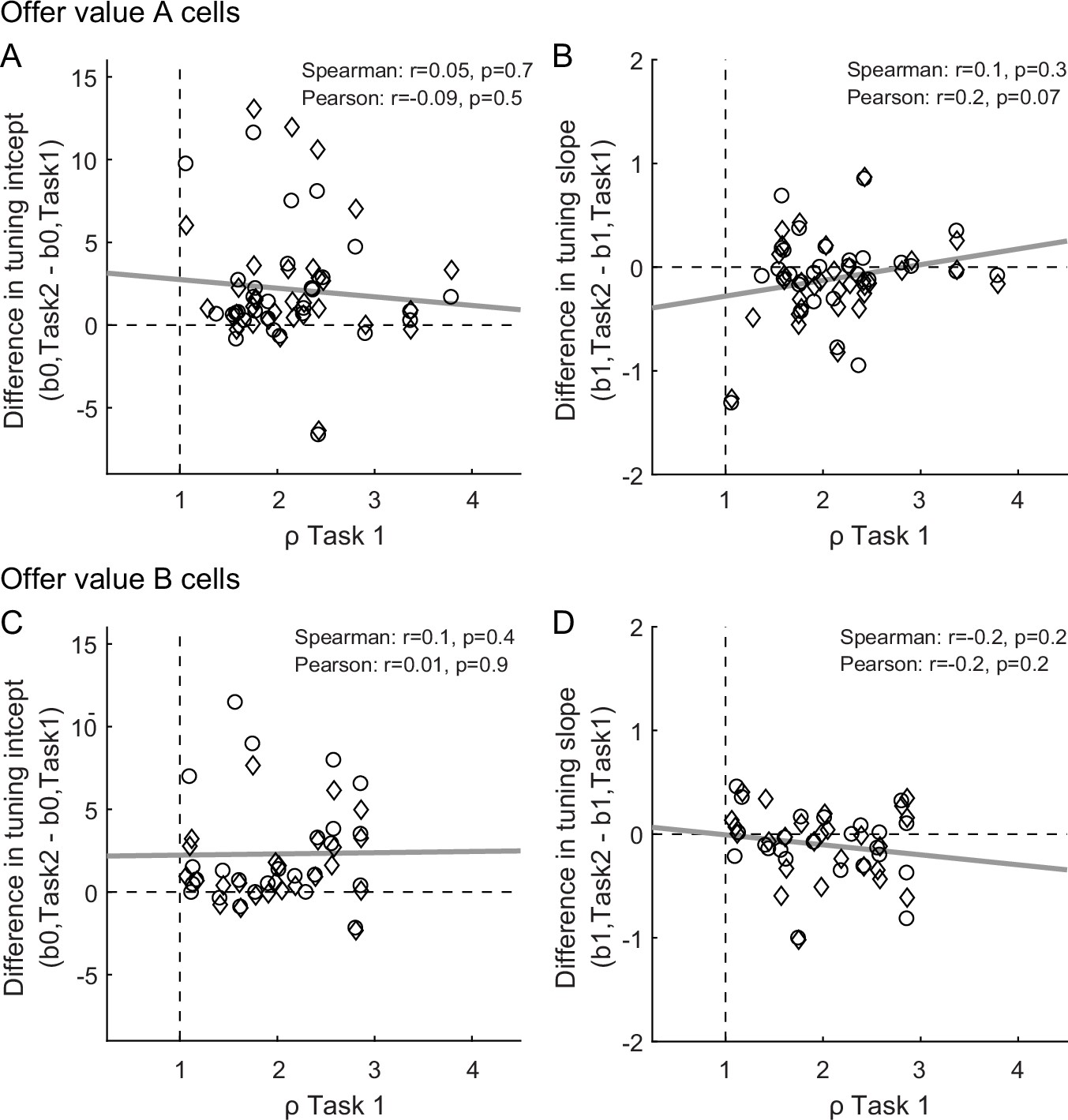
The preference bias does not reflect differences in the tuning of offer value cells.
(A, B) Offer value A cells (N = 63 cells). (C, D) Offer value B cells (N = 51 cells). Panels A and C illustrate the relation between differences in tuning intercept (y-axis) and the relative value ρTask1 (x-axis); panels B and D illustrate the relation between differences in tuning slope (y-axis) and ρTask1 (x-axis). For each offer value cell, we examined one time window (post-offer) in Task 1 and two time windows (post-offer1 and post-offer2) in Task 2. In each panel, circles and diamonds refer to post-offer1 and post-offer2 time windows, respectively. Only cells presenting significant tuning in the relevant time windows were included in the analysis (see Methods). Exact p values are indicated in each panel and gray lines are from linear regressions. These analyses did not reveal any significant correlation.
Figure 8
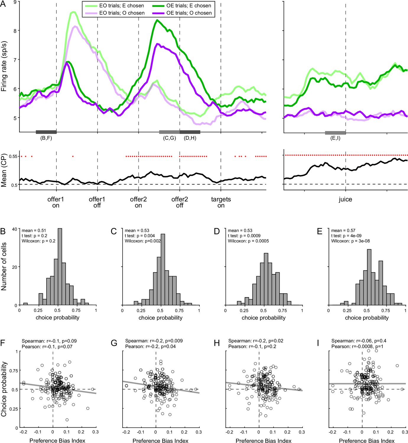
Preference bias and choice probability (CP) in chosen juice cells.
(A) Profiles of activity and CP (N = 160 cells). On the top, separate traces are activity profiles for EO trials (dark colors) and OE trials (light colors), separately for E chosen (blue) and O chosen. On the bottom the trace is the mean(CP) computed for OE trials in 100-ms sliding time windows (25-ms steps). Red dots indicate that mean(CP) was significantly >0.5 (p < 0.001; t-test). Value comparison typically takes place shortly after the onset of offer2. (B–E) Distribution of CP in four 250-ms time windows. The time windows used for this analysis are indicated in panel A. (F–I) Correlation between CP and preference bias index. Each panel corresponds to the histogram immediately above it. CPs are plotted against the preference bias index (PBI), which quantifies the preference bias independently of the juice types. Each symbol represents one cell and the line is from a linear regression. CP and PBI were negatively correlated immediately before and after offer2 onset, but not later in the trial. This pattern suggests that the preference bias emerged late in the trial, when decisions were not finalized shortly after offer2 presentation.
Author response image 1
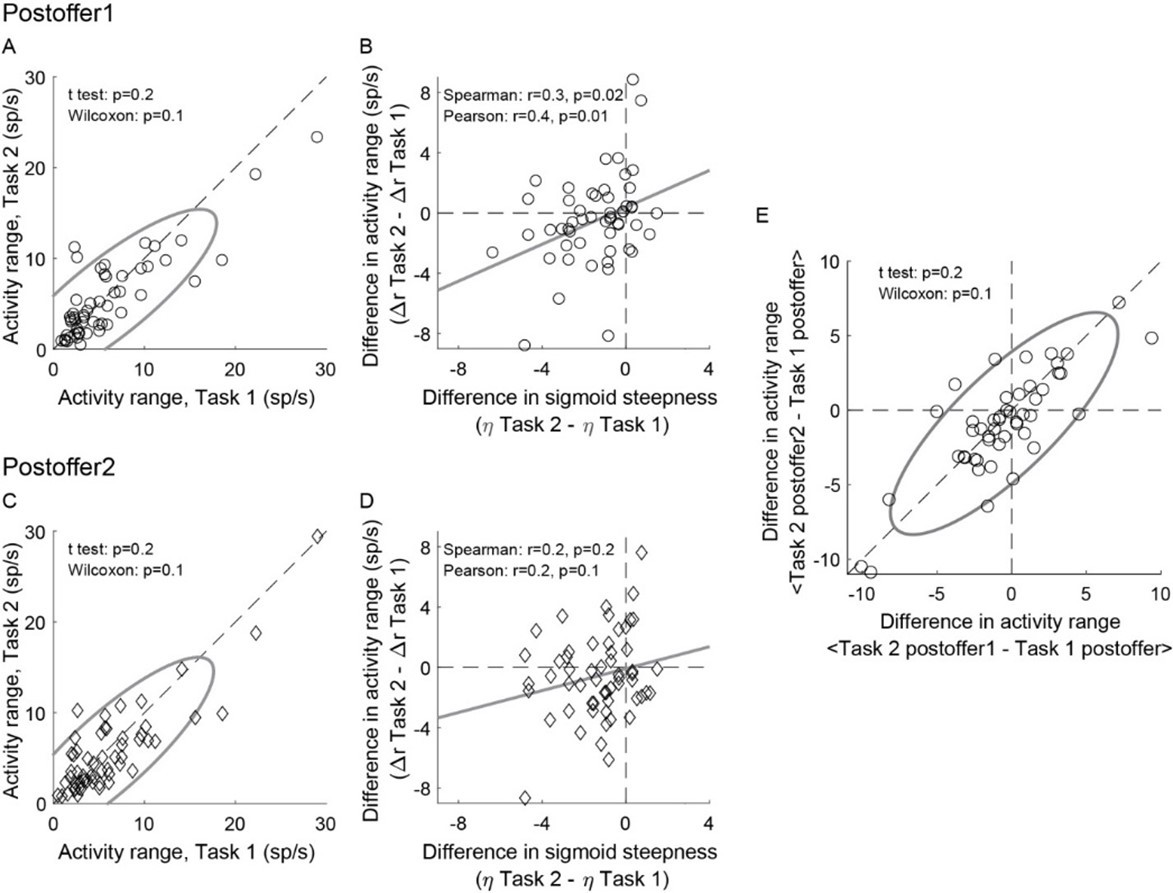
Weaker offer value signals in Task 2, population analysis in individual time windows.
(AB) Post-offer1 time window (N = 53 offer value cells). (CD) Post-offer2 time window (N = 56 offer value cells). Panel A-D are in the same format as Figure 4EF. (E) Comparing the effect across time windows. X- and y-axis represent ΔARpost-offer1 and ΔARpost-offer2, respectively. Across the population, the two measures were statistically indistinguishable.
Author response image 2
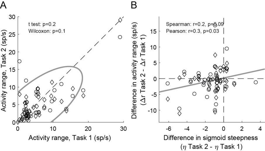
Weaker offer value signals in Task 2, population analysis based on a neuronal classification relying only on Task 2 (N = 74 offer value cells).
Panel A and B are in the same format as Figure 4EF.
Author response image 3
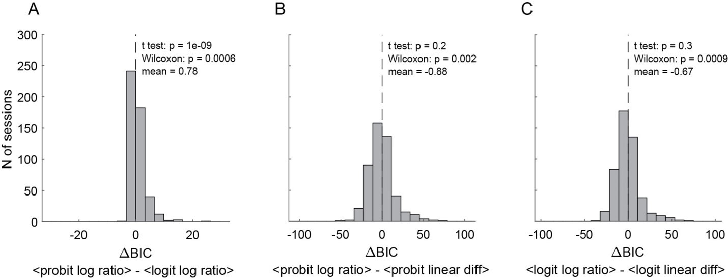
Comparing behavioral models (N = 241 sessions, pooled Task 1 and Task 2).
(A) BIC difference between probit regression with log ratio vs.. logit regression with log ratio. (B) BIC difference between probit regression with log ratio vs.. probit regression with linear difference. (C) BIC difference between logit regression with log ratio vs.. logit regression with linear difference. Smaller BIC indicates better fitting goodness, therefore negative BIC difference indicates the former model was better and vis versa. Altogether, logit regression with log quantity ratio shows the best goodness of fit. Individual data from Task 1 or Task 2 alone show similar results (not shown).
Author response image 4
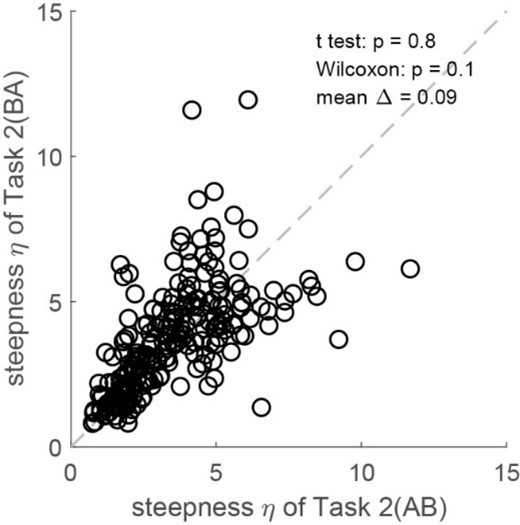
No steepness difference between AB and BA trials in Task 2 (N = 241 sessions, pooled two monkeys).
Tables
Table 1
Neuronal encoding of decision variables in the two choice tasks.
The table summarizes the results of a previous report (Shi et al., 2022a). Under simultaneous offers, different groups of orbitofrontal cortex (OFC) neurons encode different decision variables, each with positive or negative sign (indicated here with + and −). In first approximation, each cell encodes the same variable across time windows. Under sequential offers, OFC neurons encode different variables in different time windows. However, the vast majority of them present one of eight specific patterns of variables, referred to as variable ‘sequences’ and detailed here. Furthermore, there is a clear correspondence between neurons encoding a particular variable in Task 1 and neurons encoding a particular sequence in Task 2. Hence, we can refer to different cell groups in OFC using the standard nomenclature originally defined for Task 1.
| Task 1 | Task 2 | ||
|---|---|---|---|
| Post-offer1 | Post-offer2 | Post-juice | |
| offer value A + | offer value A | AB + | offer value A | BA + | chosen value A + |
| offer value A − | offer value A | AB − | offer value A | BA − | chosen value A − |
| offer value B + | offer value B | BA + | offer value B | AB + | chosen value B + |
| offer value B − | offer value B | BA - | offer value B | AB − | chosen value B − |
| chosen juice A | AB | BA + | AB | BA − | chosen juice A |
| chosen juice B | AB | BA − | AB | BA + | chosen juice B |
| chosen value + | offer value1 + | offer value2 + | chosen value + |
| chosen value − | offer value1 − | offer value2 − | chosen value − |
Additional files
Download links
A two-part list of links to download the article, or parts of the article, in various formats.
Downloads (link to download the article as PDF)
Open citations (links to open the citations from this article in various online reference manager services)
Cite this article (links to download the citations from this article in formats compatible with various reference manager tools)
Neuronal origins of reduced accuracy and biases in economic choices under sequential offers
eLife 11:e75910.
https://doi.org/10.7554/eLife.75910


