New insights into anatomical connectivity along the anterior–posterior axis of the human hippocampus using in vivo quantitative fibre tracking
- School of Biomedical Engineering, Faculty of Engineering, The University of Sydney, Australia
- Brain and Mind Centre, The University of Sydney, Australia
- School of Psychology, Faculty of Science, The University of Sydney, Australia
- Faculty of Medicine and Health Translational Research Collective, The University of Sydney, Australia
- Sydney Imaging, University of Sydney, Australia
Figures
Figure 1 with 1 supplement
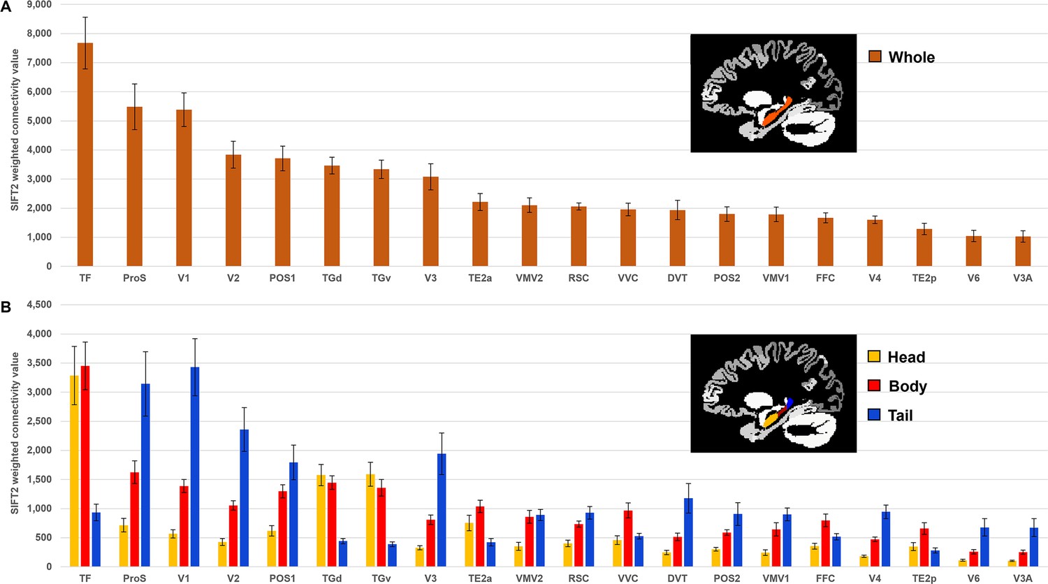
Twenty cortical brain areas with the highest degree of anatomical connectivity with the hippocampus.
(A) Histogram plotting the mean structural connectivity (n=10; given by the sum of SIFT2-weighted values) associated with the 20 cortical areas most strongly connected with the whole hippocampus (excluding medial temporal lobe [MTL] areas; see Figure 1—figure supplement 1 for MTL values). Error bars represent the standard error of the mean. (B) Histogram plotting the corresponding mean SIFT2-weighted values associated with anterior (yellow), body (red), and tail (blue) portions of the hippocampus for the 20 most strongly connected cortical areas presented in (A). Errors bars represent the standard error of the mean.
Figure 1—figure supplement 1
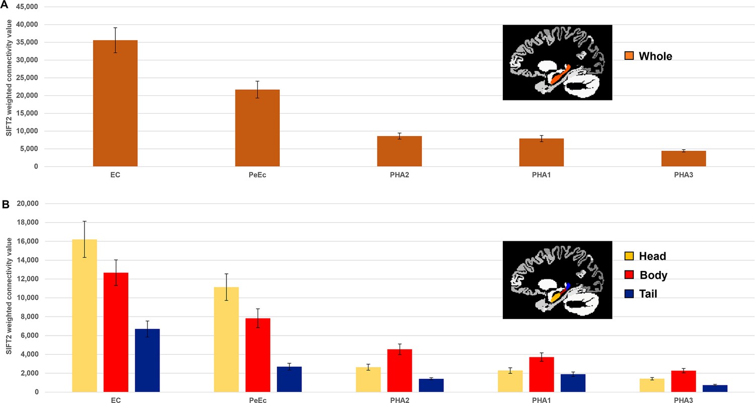
Medial temporal lobe (MTL) cortices anatomical connectivity with the hippocampus.
(A) Histogram plotting the mean structural connectivity (n=10; given by the sum of SIFT2-weighted values) associated with MTL cortical areas connected with the whole hippocampus. Error bars represent the standard error of the mean. (B) Histogram plotting the corresponding mean SIFT2-weighted values associated with anterior (yellow), body (red), and tail (blue) portions of the hippocampus for MTL cortical areas presented in (A). Errors bars represent the standard error of the mean.
Figure 2 with 4 supplements
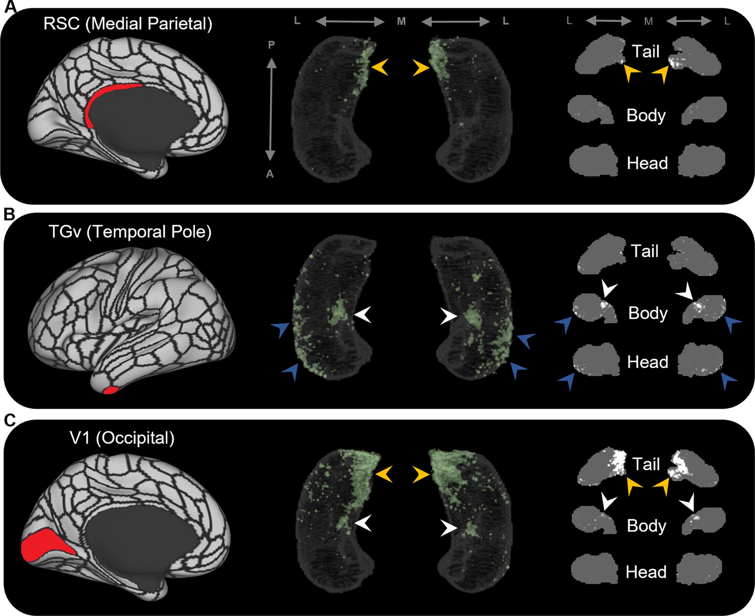
Representative examples of the spatial distribution of endpoint density within the hippocampus for different cortical brain areas.
Representative examples of the location of endpoint densities associated with RSC in the medial parietal lobe (A), TGv in the temporal pole (B), and V1 in the occipital lobe (C). In each panel, the location of the relevant brain area is indicated in red on the brain map (left); a 3D-rendered representation of the bilateral group-level hippocampus mask is presented (middle; transparent grey) overlaid with the endpoint density map associated with each brain area (green); representative slices of the head, body, and tail of the hippocampus are displayed in the coronal plane (right; grey) and overlaid with endpoint density maps (white). Note that the spatial distribution of endpoint density within the hippocampus associated with each brain area differs along both the anterior–posterior and medial–lateral axes of the hippocampus. RSC and V1 displayed greatest endpoint density in the posterior medial hippocampus (yellow arrows in A, C). In contrast, TGv displayed greatest endpoint density in the anterior lateral hippocampus and in a circumscribed region in the anterior medial hippocampus (blue and white arrows, respectively, in B). Area V1 also expressed endpoint density in a circumscribed region in the anterior medial hippocampus (white arrows in C). A, anterior; P, posterior; M, medial; L, lateral.
Figure 2—figure supplement 1
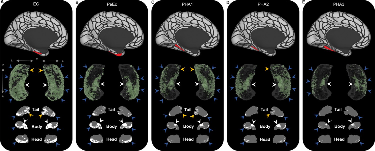
Representative examples of the spatial distribution of endpoint density within the hippocampus for medial temporal lobe (MTL) brain areas.
Representative examples of the location of endpoint densities associated with EC (A), PeEc (B), PHA1 (C), PHA2 (D), and PHA3 (E). In each panel, the location of the relevant brain area is indicated in red on the brain map (top); a 3D-rendered representation of the bilateral group-level hippocampus mask (middle; transparent grey) is presented overlaid with the endpoint density map associated with each brain area (green); representative slices of the head, body, and tail of the hippocampus are displayed in the coronal plane (bottom; grey) and overlaid with endpoint density maps (white). Note that, as expected, the spatial distribution of endpoint density associated with MTL cortical areas is denser than that observed for non-MTL cortical areas (compare with Figure 2—figure supplements 2–4). EC displayed high endpoint density throughout the hippocampus (A). PeEc (B) and PHA3 (E) displayed the greatest endpoint density along the anterior–posterior extent of the lateral hippocampus (blue arrows) and in a circumscribed region in the anterior medial hippocampus (white arrows). PeEc and PHA3 showed little endpoint density in the posterior medial hippocampus. PHA1 (C) and PHA2 (D) displayed high endpoint density along the anterior–posterior extent of the lateral hippocampus (blue arrows), in the anterior medial hippocampus (white arrows) and, in contrast to PeEc and PHA3, in the posterior medial hippocampus (yellow arrows). A, anterior; P, posterior; M, medial; L, lateral.
Figure 2—figure supplement 2
Representative examples of the spatial distribution of endpoint density within the hippocampus associated with the five most highly connected medial parietal brain areas.
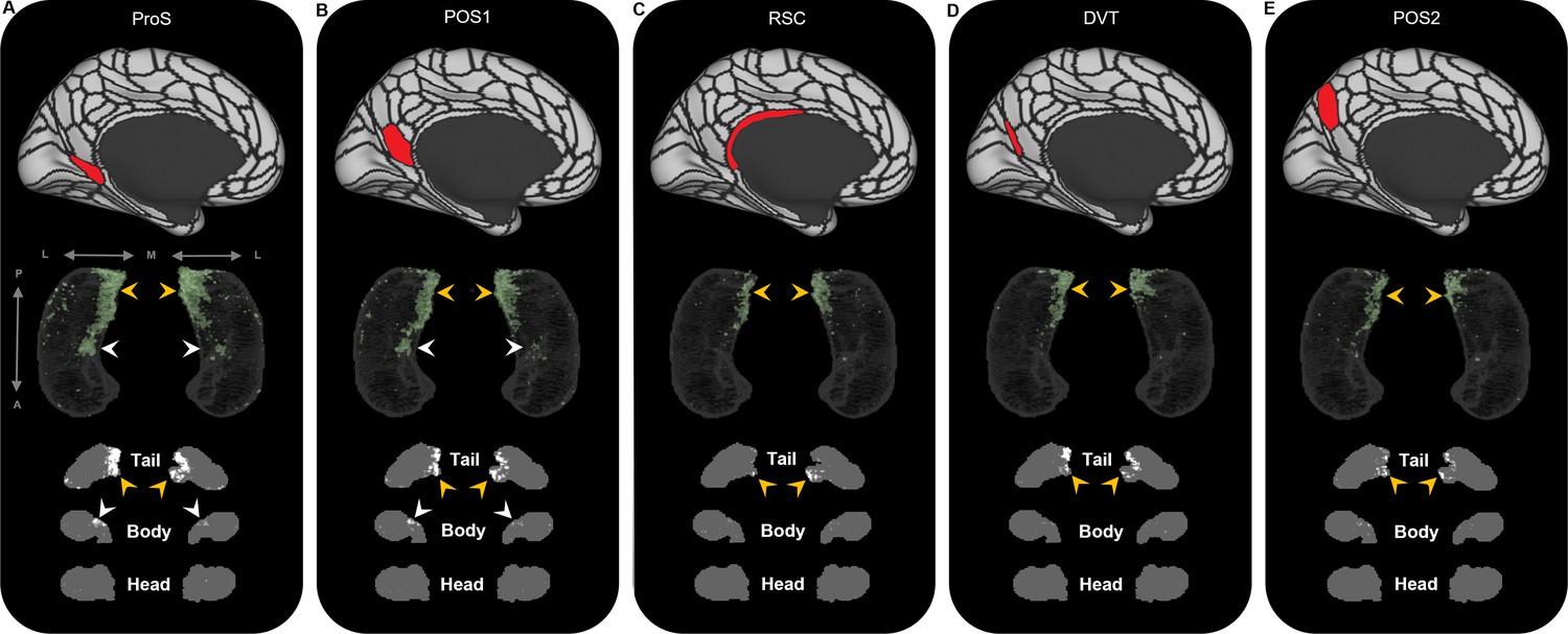
Representative examples of the location of endpoint densities associated with ProS (A), POS1 (B), RSC (C), DVT (D), and POS2 (E). In each panel, the location of the relevant brain area is indicated in red on the brain map (top); a 3D-rendered representation of the bilateral group-level hippocampus mask (middle; transparent grey) is presented overlaid with the endpoint density map associated with each brain area (green); representative slices of the head, body, and tail of the hippocampus are displayed in the coronal plane (bottom; grey) and overlaid with endpoint density maps (white). Note that the spatial distribution of endpoint density within the hippocampus associated with each of these medial parietal brain areas is primarily localised to the posterior medial hippocampus (yellow arrows in panels A–E). ProS and POS1 also display clusters of endpoint density in a circumscribed region in the anterior medial hippocampus (white arrows in panels A and B). A, anterior; P, posterior; M, medial; L, lateral.
Figure 2—figure supplement 3
Representative examples of the spatial distribution of endpoint density within the hippocampus associated with the five most highly connected non-medial temporal lobe (non-MTL) temporal brain areas.
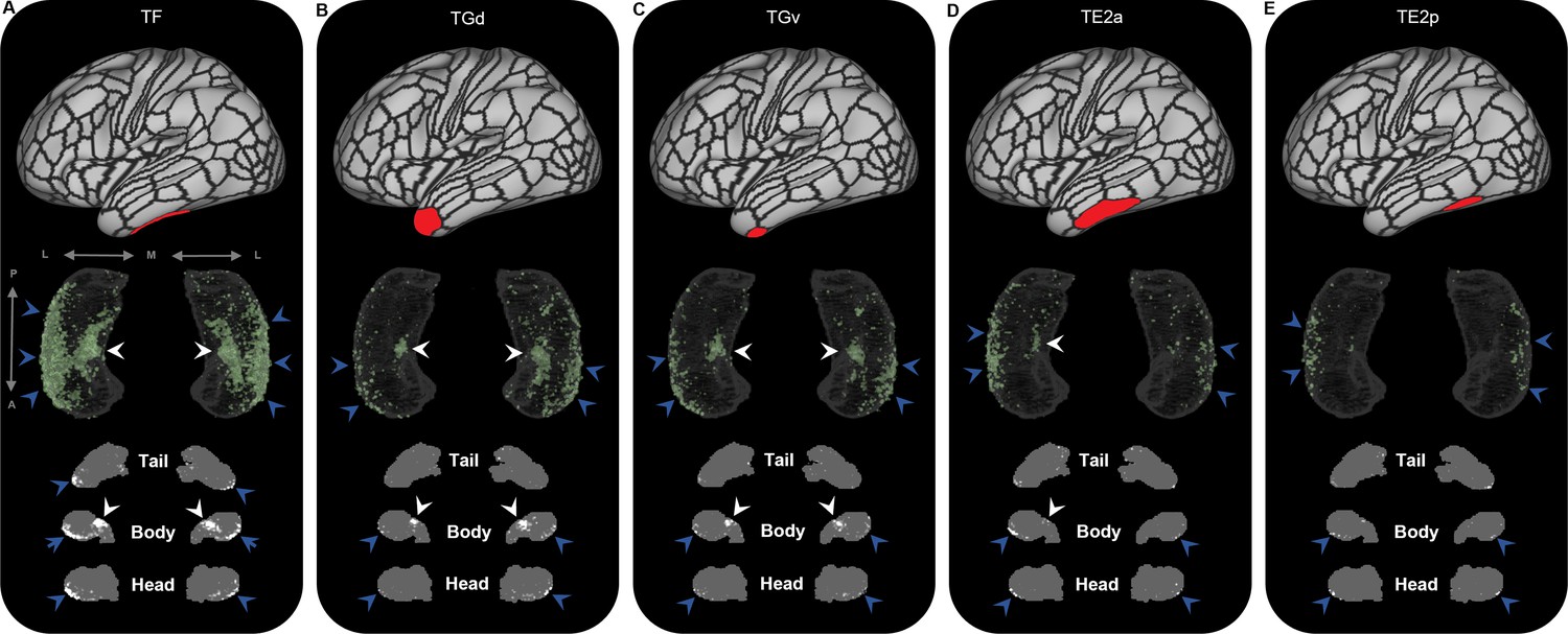
Representative examples of the location of endpoint densities associated with TF (A), Gd (B), TGv (C), TE2a (D), and TE2p (E). In each panel, the location of the relevant brain area is indicated in red on the brain map (top); a 3D-rendered representation of the bilateral group-level hippocampus mask (middle; transparent grey) is presented overlaid with the endpoint density map associated with each brain area (green); representative slices of the head, body, and tail of the hippocampus are displayed in the coronal plane (bottom; grey) and overlaid with endpoint density maps (white). Note that the spatial distribution of endpoint density within the hippocampus associated with each of these temporal brain areas is primarily localised to portions of the lateral hippocampal head and body (blue arrows in panels A–E) and a circumscribed region in the anterior medial hippocampus (white arrows in panels A–D). A, anterior; P, posterior; M, medial; L, lateral.
Figure 2—figure supplement 4
Representative examples of the spatial distribution of endpoint density within the hippocampus associated with the five most highly connected occipital brain areas.
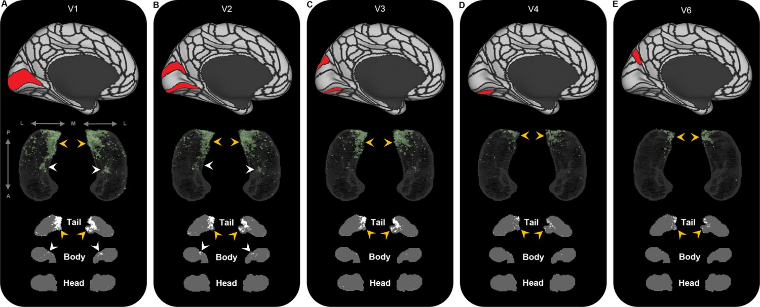
Representative examples of the location of endpoint densities associated with V1 (A), V2 (B), V3 (C), V4 (D), and V6 (E). In each panel, the location of the relevant brain area is indicated in red on the brain map (top); a 3D- rendered representation of the bilateral group-level hippocampus mask (middle; transparent grey) is presented overlaid with the endpoint density map associated with each brain area (green); representative slices of the head, body, and tail of the hippocampus are displayed in the coronal plane (bottom; grey) and overlaid with endpoint density maps (white). Note that the spatial distribution of endpoint density within the hippocampus associated with each of these occipital brain areas is primarily localised to the posterior medial hippocampus (yellow arrows in panels A–E). V1 and V2 also display clusters of endpoint density in a circumscribed region in the anterior medial hippocampus (white arrows in panels A and B). A, anterior; P, posterior; M, medial; L, lateral.
Figure 3
Averaged endpoint density maps for anatomically related brain areas.
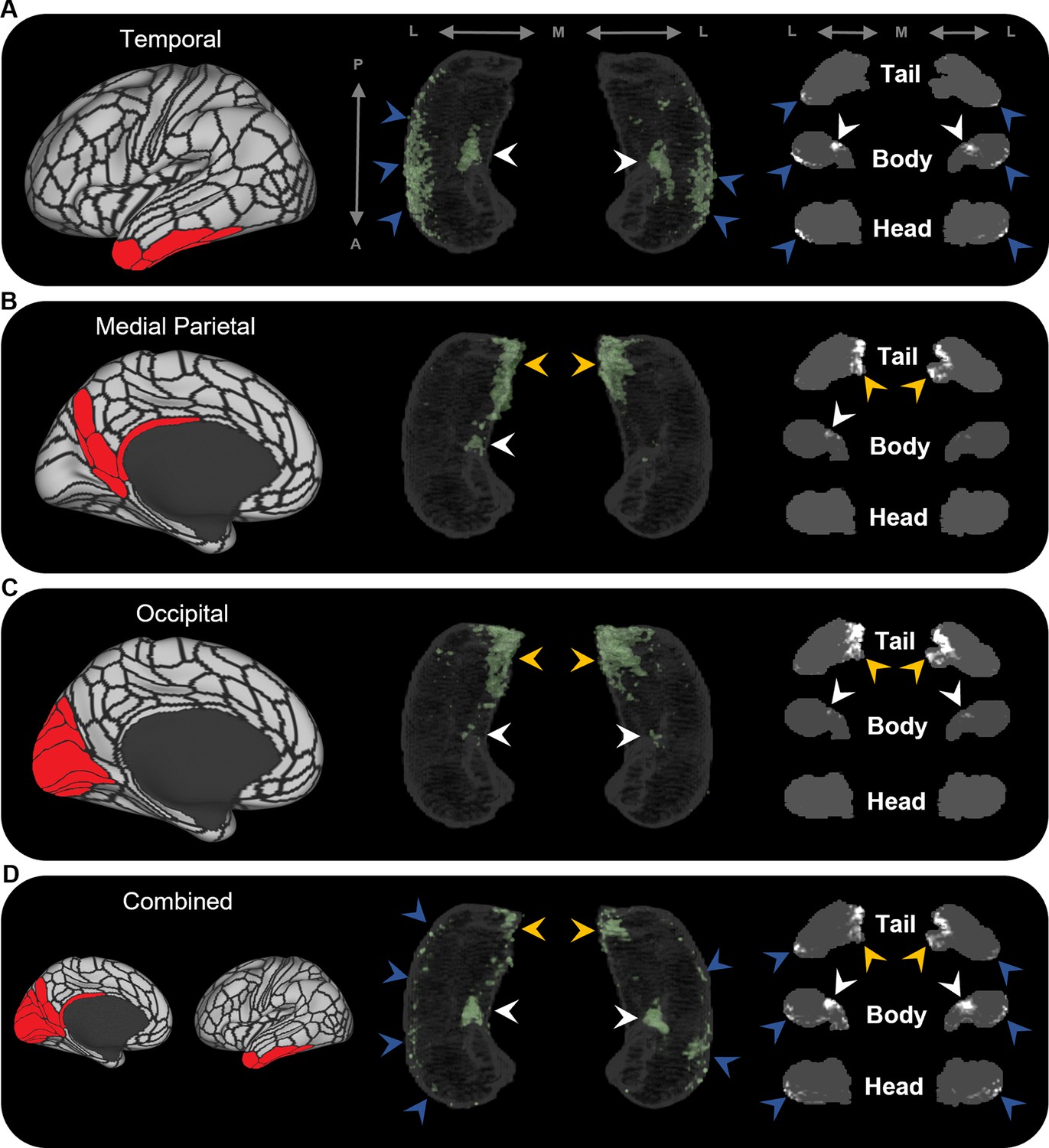
We averaged the endpoint density maps for the mostly highly connected brain areas in temporal (A; TF, TGd, TGv, TE2a, TE2p), medial parietal (B; ProS, POS1, RSC, DVT, POS2), and occipital (C; V1–4, V6, V3a) cortices and each of these regions combined (D). In each panel, the location of the relevant brain areas are indicated in red on the brain map (left); a 3D-rendered representation of the bilateral group-level hippocampus mask is presented (middle; transparent grey) overlaid with the endpoint density map associated with each collection of brain areas; representative slices of the head, body, and tail of the hippocampus are displayed in the coronal plane (right; grey) and overlaid with endpoint density maps (white). Average endpoint density associated with temporal areas (A) was primarily localised along the anterior lateral hippocampus and a circumscribed region in the anterior medial hippocampus (blue and white arrows, respectively). Average endpoint density associated with medial parietal (B) and occipital (C) areas was primarily localised to the posterior medial hippocampus (yellow arrows) and, to a lesser degree, circumscribed regions in the anterior medial hippocampus (white arrows). Average endpoint density associated with these temporal, medial parietal, and occipital brain areas combined (D) was localised to circumscribed regions in the posterior and anterior medial hippocampus (yellow and white arrows, respectively) and in punctate clusters along the anterior–posterior extent of the lateral hippocampus (blue arrows), suggesting that these specific regions within the hippocampus are highly connected with multiple cortical areas. A, anterior; P, posterior; M, medial; L, lateral.
Figure 4 with 1 supplement
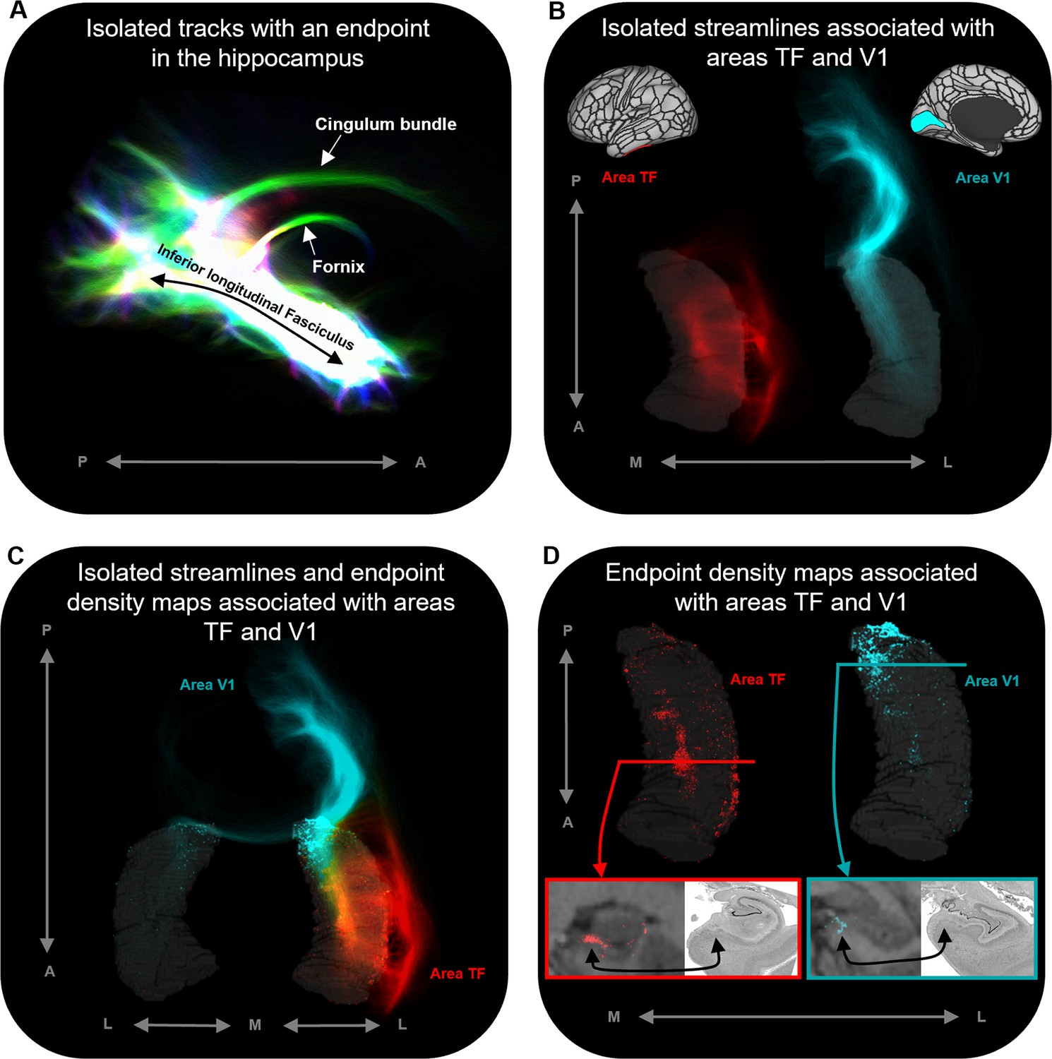
Representative examples of single-subject analysis.
(A) 3D rendering of the hippocampus tractogram for a single participant showing isolated tracks with an endpoint in the hippocampus viewed in the sagittal plane (displayed with transparency; high intensity represents high density of tracks). (B) 3D-rendered left hippocampus masks (transparent grey) for the same participant overlaid with isolated streamlines associated with the left hemisphere areas TF (red) and V1 (turquoise). The location of areas TF and V1 is indicated on the brain maps (top). (C) 3D-rendered bilateral hippocampus mask for the same participant (transparent grey) overlaid with isolated streamlines and endpoint density maps associated with the left hemisphere areas TF (red) and V1 (turquoise). Note that, while streamlines associated with areas TF and V1 are primarily ipsilateral in nature, streamlines associated with V1 also project to the contralateral hippocampus. (D) 3D-rendered left hippocampus masks (transparent grey) for the same participant overlaid with endpoint density maps associated with areas TF (red) and V1 (turquoise). For TF and V1, we present a coronal section of the T1-weighted structural image overlaid with the endpoint density maps and a corresponding slice of postmortem hippocampal tissue (from a different subject) for anatomical comparison (bottom). For both TF (red border; level of the uncal apex) and V1 (turquoise border; level of the hippocampal tail), endpoint density is primarily localised to a circumscribed region in the medial hippocampus aligning with the location of the distal subiculum/proximal presubiculum (black arrows; also see Figure 5A). A, anterior; P, posterior; M, medial; L, lateral.
© 2019, The BigBrain. Post-mortem images are reproduced from the BigBrain Project (Amunts et al., 2013). The images are published under the terms of the Creative Commons NonCommercial-ShareAlike 4.0 International license CC BY-NC-SA 4.0
Figure 4—figure supplement 1
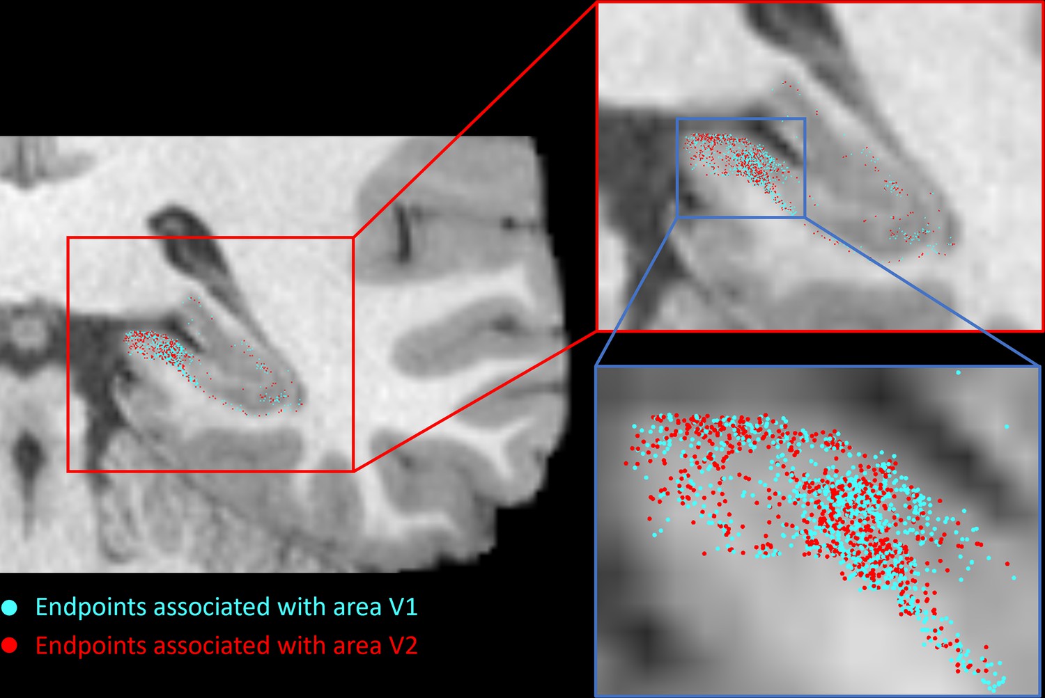
Cortical areas display both overlapping and spatially unique endpoints within specific regions of the hippocampus.
Group-level analysis revealed that specific cortical areas (e.g. V1 and V2) showed preferential connectivity with overlapping regions within the hippocampus (e.g. within the posterior medial hippocampus; see Figure 2—figure supplement 4 for an example). However, at the single-participant level, individual endpoints associated with each of these areas display both overlapping and spatially unique patterns (compare the spatial distribution of streamline endpoints associated with V1 [cyan] and V2 [red] in the posterior medial hippocampus). This suggests that, while different cortical areas display overlapping patterns of connectivity within specific regions of the hippocampus, subtle differences in how each cortical region connects within these areas of overlap likely exist.
Figure 5
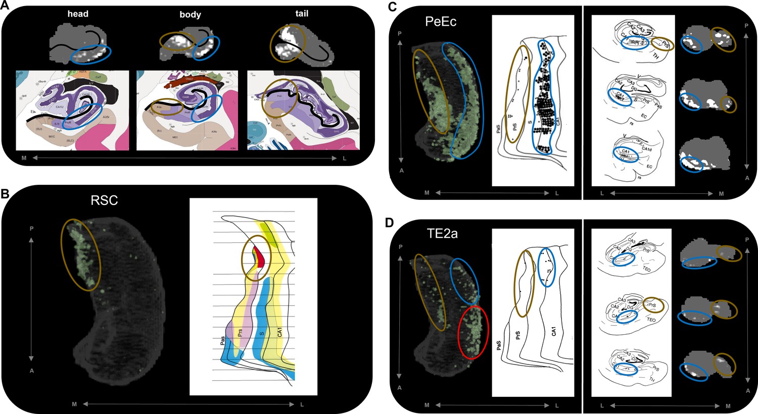
Anatomical location of endpoint densities within the hippocampus and comparison with results of non-human primate studies.
(A) Representative slices of the head (left), body (middle), and tail (right) of the hippocampus displayed in the coronal plane (grey) and overlaid with group-level endpoint density maps associated with areas TF (head and body; white) and V1 (tail; white). Schematic representations of roughly equivalent slices of the hippocampus showing hippocampal subfields are displayed below each slice. Schematic representations were taken from the Allen Adult Human Brain Atlas website (https://atlas.brain-map.org/; Ding et al., 2016; Allen Institute for Brain Science, 2004). The vestigial hippocampal sulcus (black line) is overlaid on the hippocampus masks and schematic diagrams to aid comparison. Note that the endpoint density in the lateral hippocampus (blue ellipsoids) aligns with the location of the distal CA1/proximal subiculum. Endpoint density in the medial hippocampus (brown ellipsoids) aligns with the location of distal subiculum/proximal presubiculum. (B–D) 3D-rendered representations of the group-level hippocampus mask (left; transparent grey) are overlaid with endpoint density maps (green) associated with RSC (B), PeEc (C), and TE2a (D). Schematic representations of the macaque hippocampus (right; images reproduced with permission from Insausti and Muñoz, 2001) show the location of labelled cells following retrograde tracer injection into the RSC (B; red), PeEc (C; black points), and TE2a (D; black points) (Insausti and Muñoz, 2001). The right panel of (C) and (D) displays slices of the macaque hippocampus in the coronal plane displaying the location of labelled cells (black points) and roughly equivalent slices of human hippocampus in the coronal plane (grey) overlaid with endpoint density maps (white). Note that labelled cells and endpoint density in the macaque and human respectively are localised to similar regions along the anterior–posterior and medial (brown ellipsoids) – lateral (blue ellipsoids) axes of the hippocampus. However, areas of difference also exist (D; red ellipsoid). M, medial; L, lateral; A, anterior; P, posterior.
© 2016, Ding et al. Figure 5a schematic representations are reproduced from Figure 17; Level 45a (05_063), Figure 17; Level 52a (05_159) and Figure 17; Level 67a (06_083) from Ding et al., 2016 and from the Allen Adult Human Brain Atlas website. The images are published under the terms of the Creative Commons NonCommercial-NoDerivatives 4.0 International license CC BY-NC-ND 4.0
© 2001, John Wiley and Sons. Figure 5 b, c and d are reproduced from Figure 9, 6 and 5 respectively from Insausti and Muñoz, 2001 with permissions from John Wiley and Sons. It is not covered by the CC-BY 4.0 licence and further reproduction of this panel would need permission from the copyright holder.
Figure 6
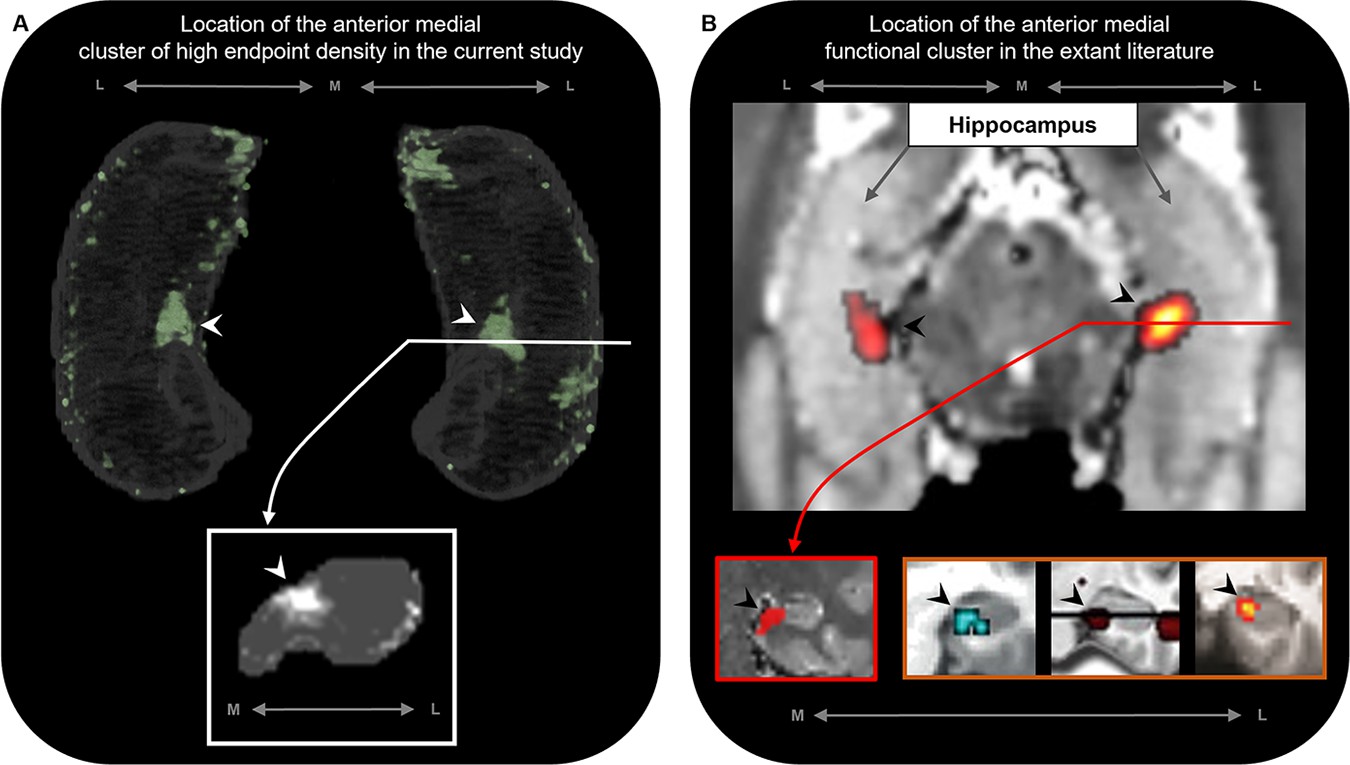
The location of the anterior medial anatomical cluster aligns with the location of a commonly observed anterior medial functional cluster.
(A) A 3D-rendered representation of the bilateral group-level hippocampus mask (top; transparent grey) is presented overlaid with the endpoint density map averaged across the most highly connected brain areas in temporal, medial parietal, and occipital cortices (green; see Figure 3D for details); a representative slice of hippocampus in the coronal plane (bottom panel; grey) at the level of the uncal apex (indicated by white line) is presented overlaid with the endpoint density map (white). (B) An axial section of a T2-weighted image (top; from a separate study) showing the bilateral hippocampus overlaid with the location of a circumscribed functional cluster observed in the anterior medial hippocampus during a functional MRI investigation of visuospatial mental imagery, reproduced from Figure 2b from Dalton et al., 2018. A representative slice of the hippocampus (bottom-left panel; red border) at the level of the uncal apex (indicated by red line) is presented to show the location of this anterior medial functional cluster in the coronal plane, reproduced from Figure 3a from Dalton et al., 2018. Circumscribed functional clusters in the anterior medial hippocampus are commonly observed in studies of ‘scene-based visuospatial cognition’ such as episodic memory, prospection and scene perception (bottom-right panel; orange border). Left image was reproduced from Figure 3 from Zeidman et al., 2015b. Middle image was reproduced from Figure 3 from Addis et al., 2012. Right image was reproduced from Figure 4a from Lee et al., 2013. Note that the location of these commonly observed functional clusters in the anterior medial hippocampus (black arrows in panel B) aligns with the location of the anatomical cluster in the anterior medial hippocampus observed in this study (white arrows in panel A). M, medial; L, lateral.
© 2012, Elsevier. Middle image is reproduced from Figure 3 from Addis et al., 2012 with permission from Elsevier. It is not covered by the CC-BY 4.0 licence and further reproduction of this panel would need permission from the copyright holder.
© 2013, Massachusetts Institute of Technology Press. Right image is reproduced from Figure 4a from Lee et al., 2013 with permission from Massachusetts Institute of Technology Press Journals. It is not covered by the CC-BY 4.0 licence and further reproduction of this panel would need permission from the copyright holder.
Figure 7 with 2 supplements
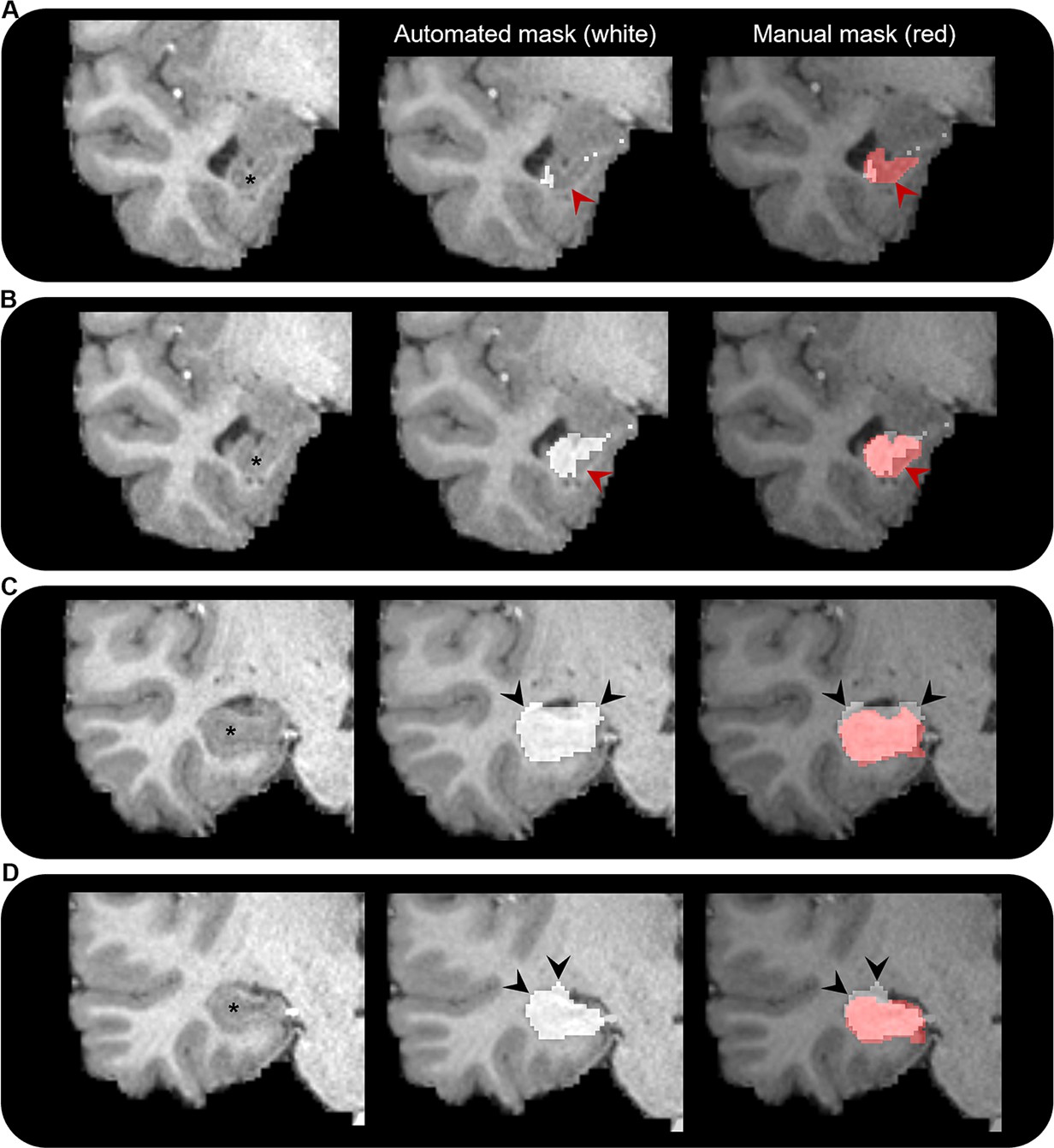
Comparison of automated and manual hippocampus segmentations.
Representative examples of the automated hippocampus mask derived from the Human Connectome Project Multi-Modal Parcellation (HCPMMP) and the manually segmented hippocampus mask. We display examples from anterior (A) to posterior (D) portions of the hippocampal head. In each panel, we present a coronal slice of the T1-weighted image focused on the right temporal lobe for a single participant (left; hippocampus indicated by *), the same image overlaid with the automated hippocampus mask derived from the HCPMMP (middle; white) and the same image overlaid with both the automated HCPMMP hippocampus mask (right; white) and the manually segmented hippocampus mask (transparent red). Note that in the anterior-most slices (A, B) the automated mask does not cover the entire extent of the hippocampus (indicated by red arrows) and in more posterior slices (C, D) the automated mask often overextends across the lateral ventricle superior to the hippocampus and into the adjacent white matter (indicated by black arrows). Streamlines making contact with these erroneous portions of the automated hippocampus mask may lead to results that are biologically implausible.
Figure 7—figure supplement 1
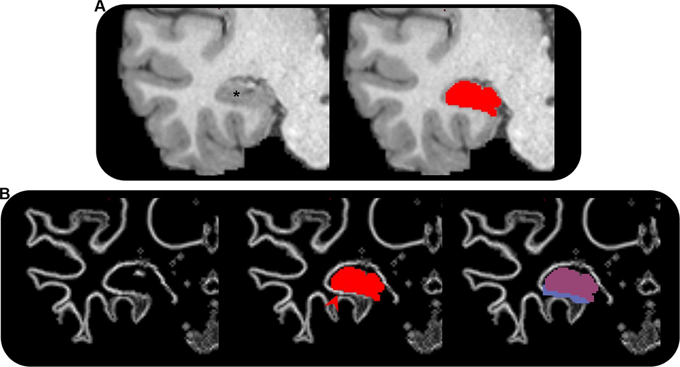
Adjustment of grey matter–white matter interface (gmwmi) underlying the hippocampus.
(A) T1-weighted structural MRI scan showing the right medial temporal lobe (left; hippocampus indicated by *) in the coronal plane for a single participant and the manually segmented hippocampus mask (red) overlaid on the T1-weighted image (right). (B) Left: the gmwmi (white line) showing the right medial temporal lobe in the coronal plane; middle: the manually segmented hippocampus mask (red) overlaid on the gmwmi. Note: portions of detected gmwmi immediately inferior to the hippocampus lie outside of the hippocampus mask (indicated by red arrow). If left unchanged, the anatomically informed tractography algorithm used in this study would terminate tracks as they reach this band, thus creating an erroneous band of track endpoints in this region, introducing misleading results. Right: the hippocampus mask (transparent red) and extended hippocampus mask (blue) overlaid on the gmwmi. Note: the extended hippocampus mask encompasses the gmwmi immediately inferior to the hippocampus. This allows streamlines to enter/leave the hippocampus here rather than terminate at the gmwmi (see ‘Materials and methods’ for detail).
Figure 7—figure supplement 2
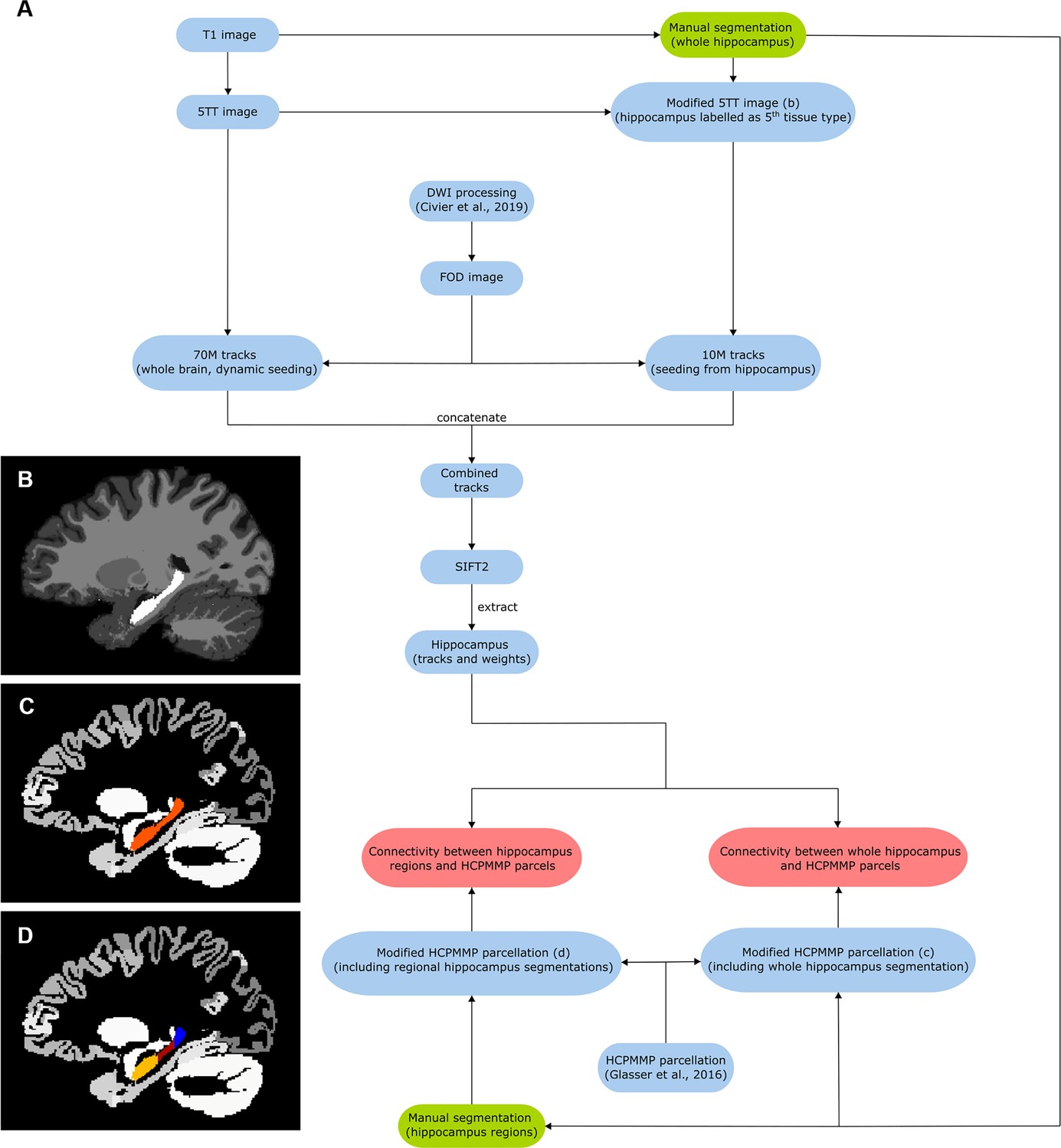
Analysis pipeline.
(A) Block diagram of the workflow. Green blocks indicate procedures that involved manual segmentation, red blocks indicate connectivity vectors/matrices from which connectivity measurements were obtained, and blue blocks indicate intermediate images. (B) Sagittal view of ‘modified 5TT’ image containing the manually segmented hippocampus labelled as ‘5th tissue type’ (i.e. no anatomical prior for tracking) shown in white. (C) Sagittal view of modified parcellation image containing the whole-hippocampus mask (shown in orange). (D) Sagittal view of modified parcellation image containing the regional hippocampus masks (head, body, and tail shown in yellow, red, and blue, respectively).
Tables
Table 1
Twenty cortical brain areas (excluding medial temporal lobe) with the highest degree of anatomical connectivity with the whole hippocampus.
| Cortical area | Location of area | Whole hippocampus | ||
|---|---|---|---|---|
| Mean SIFT2-weighted value(connectivity strength; n=10) | Standard error of mean | Percent of all cortical connections accounted for by area(percent of cortical connections excluding MTL areas) | ||
| TF | Lateral temporal cortex | 7673 | 886 | 5.10 (10.61) |
| ProS | Medial parietal cortex (including posterior cingulate) | 5483 | 784 | 3.64 (7.58) |
| V1 | Early visual cortex (occipital) | 5385 | 579 | 3.58 (7.45) |
| V2 | Early visual cortex (occipital) | 3840 | 462 | 2.55 (5.31) |
| POS1 | Medial parietal cortex (including posterior cingulate) | 3712 | 424 | 2.47 (5.13) |
| TGd | Temporal pole | 3465 | 288 | 2.30 (4.79) |
| TGv | Temporal pole | 3337 | 313 | 2.22 (4.61) |
| V3 | Early visual cortex (occipital) | 3079 | 450 | 2.05 (4.26) |
| TE2a | Lateral temporal cortex | 2214 | 288 | 1.47 (3.06) |
| VMV2 | Ventral stream visual cortex | 2105 | 247 | 1.40 (2.91) |
| RSC | Medial parietal cortex (including posterior cingulate) | 2063 | 121 | 1.37 (2.85) |
| VVC | Ventral stream visual cortex | 1956 | 220 | 1.30 (2.71) |
| DVT | Medial parietal cortex (including posterior cingulate) | 1939 | 335 | 1.29 (2.68) |
| POS2 | Medial parietal cortex (including posterior cingulate) | 1802 | 248 | 1.20 (2.49) |
| VMV1 | Ventral stream visual cortex | 1788 | 248 | 1.19 (2.47) |
| FFC | Ventral stream visual cortex | 1670 | 172 | 1.11 (2.31) |
| V4 | Early visual cortex (occipital) | 1601 | 127 | 1.06 (2.21) |
| TE2p | Lateral temporal cortex | 1288 | 198 | 0.86 (1.78) |
| V6 | Dorsal stream visual cortex | 1050 | 195 | 0.70 (1.45) |
| V3A | Dorsal stream visual cortex | 1029 | 197 | 0.68 (1.42) |
-
Column 1 displays cortical areas as defined by the Human Connectome Project Multi-Modal Parcellation (HCPMMP) scheme and ordered by strength of connectivity with the whole hippocampus (abbreviations for all cortical areas are defined in Supplementary file 3). Column 2 indicates the broader brain region within which each cortical area is located. Column 3 displays the mean SIFT2-weighted value (connectivity strength) associated with each brain area. Column 4 displays the standard error of the mean. Column 5 displays the percent of all cortical connections accounted for by each area. Values in brackets indicate the percent of cortical connections accounted for by each area when excluding medial temporal lobe (MTL) areas.
Additional files
-
Transparent reporting form
- https://cdn.elifesciences.org/articles/76143/elife-76143-transrepform1-v1.pdf
-
Supplementary file 1
Connectivity values between the cortical mantle and the whole hippocampus.
Connectivity values between the whole hippocampus and all cortical areas in the Human Connectome Project Multi-Modal Parcellation (HCPMMP) scheme are presented. Column 1 displays each broad brain region ordered by their strength of connectivity with the whole hippocampus. Column 2 displays the percent of all cortical connections accounted for by each region. Values in brackets indicate the percent of cortical connections accounted for by each region when excluding medial temporal lobe (MTL) areas. Column 3 presents the cortical areas located within each broad brain region ordered by their strength of connectivity with the whole hippocampus (abbreviations for all cortical areas are defined in Supplementary file 3). Column 4 displays the mean SIFT2 weighted value (connectivity strength) associated with each cortical area. Column 5 displays the standard error of the mean. Column 6 displays the percent of all cortical connections accounted for by each cortical area. Values in brackets indicate the percent of cortical connections accounted for by each cortical area when excluding MTL areas. Column 7 displays the rank order for each cortical area by strength of connectivity. Values in brackets indicate the rank order when excluding MTL areas.
- https://cdn.elifesciences.org/articles/76143/elife-76143-supp1-v1.docx
-
Supplementary file 2
Connectivity between the cortical mantle and the head, body, and tail of the hippocampus.
Connectivity values between the head, body, and tail of the hippocampus and all cortical brain areas included in the Human Connectome Project Multi-Modal Parcellation (HCPMMP) scheme are presented. Column 1 displays each cortical area ordered by strength of connectivity with the whole hippocampus (abbreviations for all cortical areas are defined in Supplementary file 3). Column 2 presents the broader brain region within which each cortical area is located. Column 3 displays the mean SIFT2-weighted value (connectivity strength) associated with each cortical area and the head of the hippocampus. Column 4 displays the associated standard error of the mean. Column 5 displays the mean SIFT2-weighted value (connectivity strength) associated with each cortical area and the body of the hippocampus. Column 6 displays the associated standard error of the mean. Column 7 displays the mean SIFT2-weighted value (connectivity strength) associated with each cortical area and the tail of the hippocampus. Column 8 displays the associated standard error of the mean.
- https://cdn.elifesciences.org/articles/76143/elife-76143-supp2-v1.docx
-
Supplementary file 3
List of abbreviations for all cortical brain areas in the Human Connectome Project Multi-Modal Parcellation (HCPMMP) scheme.
- https://cdn.elifesciences.org/articles/76143/elife-76143-supp3-v1.docx
-
Supplementary file 4
Connectivity between the 20 most highly connected cortical areas and the head, body, and tail of the hippocampus.
Column 1 displays cortical areas as defined by the Human Connectome Project Multi-Modal Parcellation (HCPMMP) scheme and ordered by strength of connectivity with the whole hippocampus (abbreviations for all cortical areas are defined in Supplementary file 3). Column 2 designates the portion of hippocampus (head, body, tail). Column 3 displays the mean SIFT2-weighted value (connectivity strength) between each cortical area and the head, body, and tail of the hippocampus. Column 4 displays the standard error of the mean. Column 5 displays the contrast for each paired-samples t-test. Column 6 displays the t-statistic associated with each pair. Column 7 displays the p-value associated with each pair. Column 8 indicates the significance level associated with each pair following Bonferroni correction. ***<0.001, **<0.01, *<0.05, ns, not statistically significant.
- https://cdn.elifesciences.org/articles/76143/elife-76143-supp4-v1.docx
Download links
A two-part list of links to download the article, or parts of the article, in various formats.
Downloads (link to download the article as PDF)
Open citations (links to open the citations from this article in various online reference manager services)
Cite this article (links to download the citations from this article in formats compatible with various reference manager tools)
New insights into anatomical connectivity along the anterior–posterior axis of the human hippocampus using in vivo quantitative fibre tracking
eLife 11:e76143.
https://doi.org/10.7554/eLife.76143


