Selfee, self-supervised features extraction of animal behaviors
- School of Life Sciences, IDG/McGovern Institute for Brain Research, Tsinghua University, China
- Tsinghua-Peking Center for Life Sciences, China
- Institute of Neuroscience, State Key Laboratory of Neuroscience, Chinese Academy of Sciences Center for Excellence in Brain Science and Intelligence Technology, China
- Shanghai Center for Brain Science and Brain-Inspired Intelligence Technology, China
Figures
Figure 1 with 6 supplements
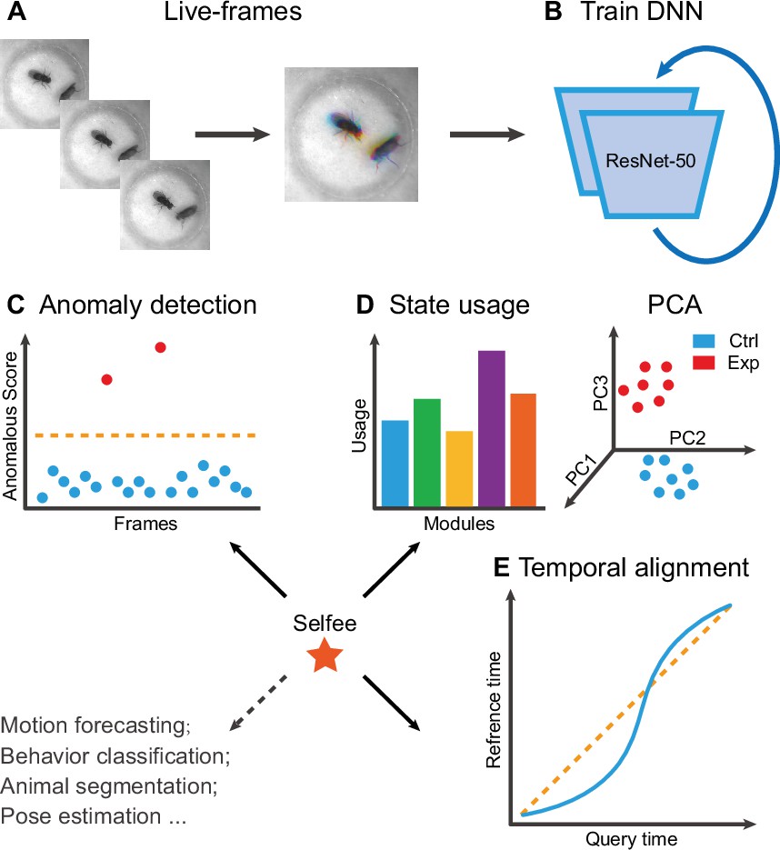
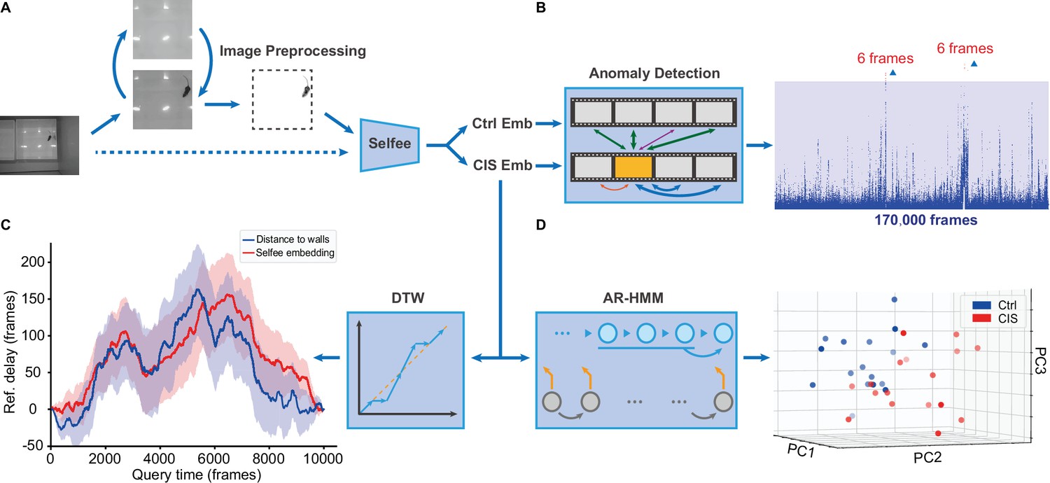
The framework of Selfee (Self-supervised Features Extraction) and its downstream applications.
(A) One live-frame is composed of three tandem frames in R, G, and B channels, respectively. The live-frame could capture the dynamics of animal behaviors. (B) Live-frames are used to train Selfee, which adopts a backbone of ResNet-50. (C, D, and E) Representations produced by Selfee could be used for anomaly detection that could identify unusual animal postures in the query video compared with the reference videos. (C) AR-HMM (autoregressive hidden Markov model) that models the local temporal characteristics of behaviors and clusters frames into modules (states) and calculates stages usages of different genotypes (D) DTW (dynamic time warping) that aligns behavior videos to reveal differences of long-term dynamics (E) and other potential tasks including behavior classification, forecasting, or even image segmentation and pose estimation after appropriately modifying and fine-tuning of the neural networks.
Figure 1—figure supplement 1
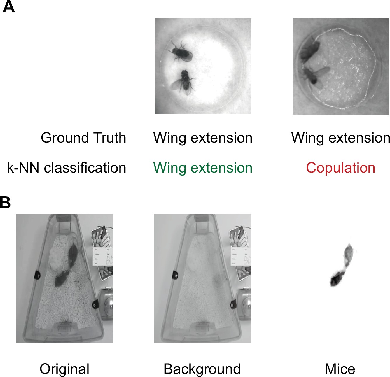
Beddings and backgrounds that affect training and inference of Selfee (Self-supervised Features Extraction).
(A) Textures on the damped filter paper would mislead Selfee to output features similar to copulation but not wing extension (ground truth). The left example showed a background that would not affect Selfee neural network, and the right example showed a background that could strongly affect classification accuracy. (B) Background inconsistency would affect the training process when Selfee was applied to mice behavior data. Therefore, backgrounds were removed from all frames to avoid potential defects. After background removal, illumination normalization was applied.
Figure 1—figure supplement 2
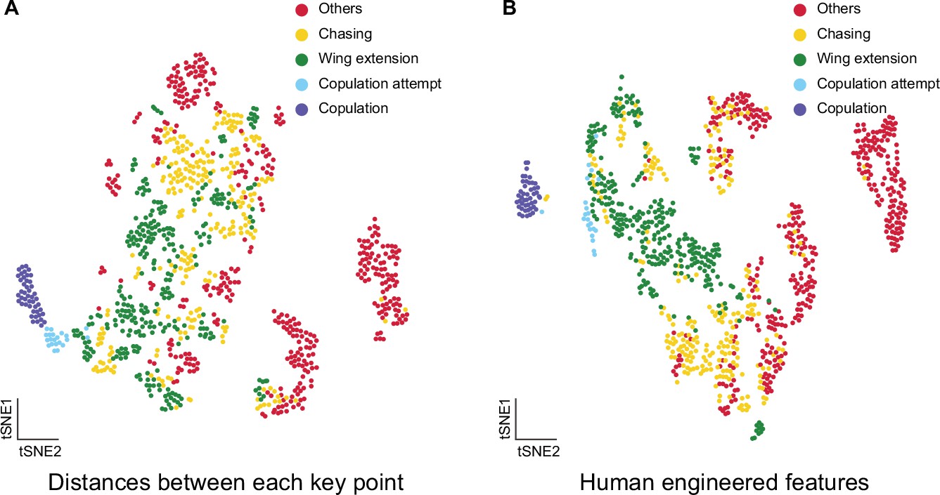
t-SNE visualization of pose estimation derived features.
(A) Visualization of fly courtship live-frames with t-SNE dimension reduction of distances between key points, including head, tail, thorax, and wings. Each dot was colored based on human annotations. Points representing non-interactive behaviors (‘others’), chasing, wing extension, copulation attempt, and copulation were colored with red, yellow, green, blue, and violet, respectively. (B) Visualization of fly courtship live-frames with t-SNE dimension reduction of human-engineered features, including male head to female tail distance, male body to female body distance, male wing angle, female wing angle, and angle between male body axis. Each dot was colored based on human annotations. Points representing non-interactive behaviors (‘others’), chasing, wing extension, copulation attempt, and copulation were colored with red, yellow, green, blue, and violet, respectively.
Figure 1—figure supplement 3
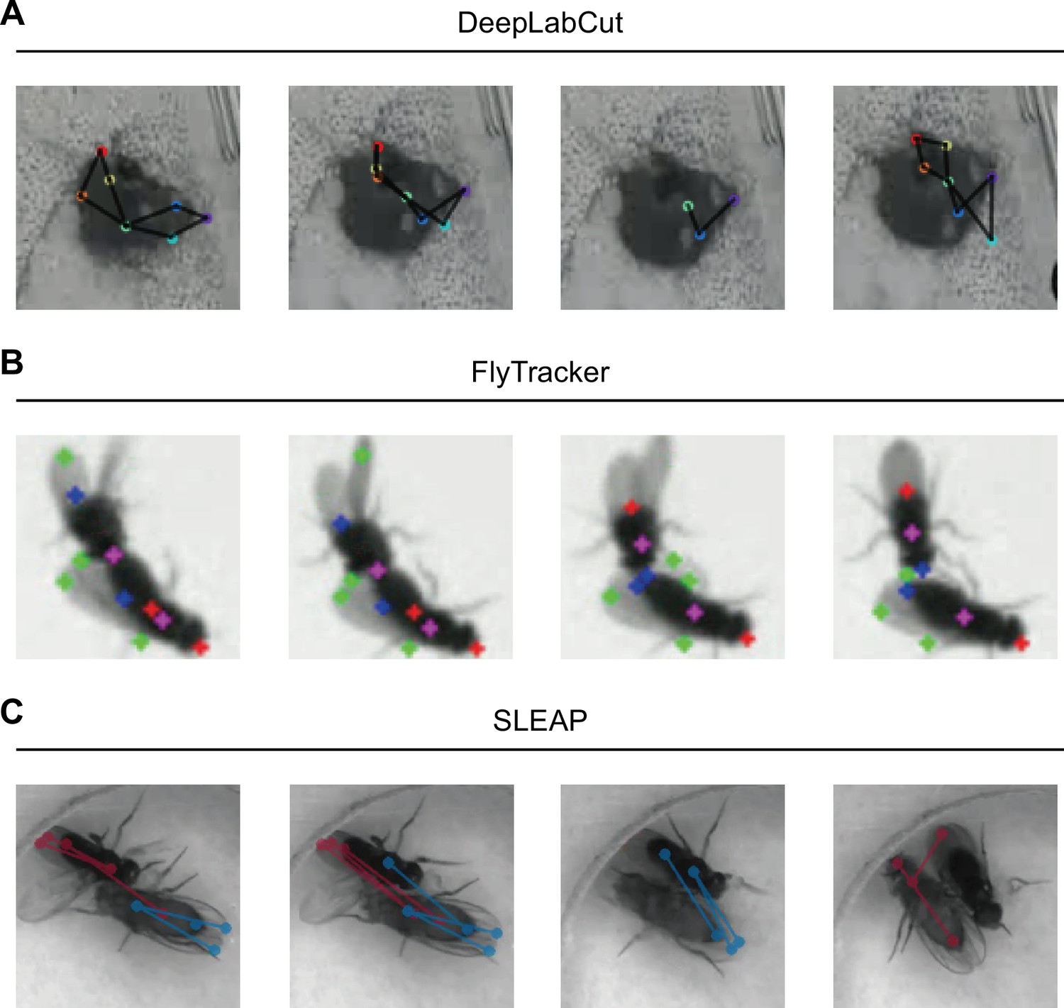
Animal tracking with DLC, FlyTracker, and SLEAP.
(A) Visualization of DLC tracking results on intensive interactions between mice during mating behavior. The nose, ears, body center, hips, and bottom were labeled. DLC tended to detect two animals as one due to occluding. (B) Visualization of FlyTracker tracking results provided in Fly-vs-Fly dataset. The head, tail, center, and wings were colored in red, blue, purple, and green, respectively. When two flies were close, wings became hard to be detected correctly. (C) Visualization of SLEAP tracking results on close interactions during fly courtship behavior. Five body parts were marked with points, including head, tail, thorax, and wings, and head to tail, thorax to wings were linked by lines. Female was labeled in red, and the male was in blue. Body parts were wrongly assigned when two animals were close.
Figure 1—video 1
Visualization of DLC tracking results on intensive interactions between mice during mating behavior.
The nose, ears, body center, hips, and bottom were labeled. DLC worked great when two animals were separated, but it tended to detect two animals as one during mounting or intromission due to occluding.
Figure 1—video 2
A tracking example of FlyTracker of Fly-vs-Fly dataset.
Visualization of FlyTracker tracking results provided in Fly-vs-Fly dataset. The head, tail, center, and wings were colored in red, blue, purple, and green, respectively. The tracking result was very competent even compared with deep learning-based methods. However, when two flies were close, wings, even bodies, became hard to be detected correctly.
Figure 1—video 3
A tracking example of SLEAP on fly courtship behavior.
Visualization of SLEAP tracking results on fly courtship behavior. Five body parts were marked with points, including head, tail, thorax, and wings, and head to tail, thorax to wings were linked by lines. Female was labeled in red, and the male was in blue. In general, the tracking result was good. However, body parts were wrongly assigned when two animals were close, and performance was significantly impaired during copulation attempt and copulation.
Figure 2 with 1 supplement
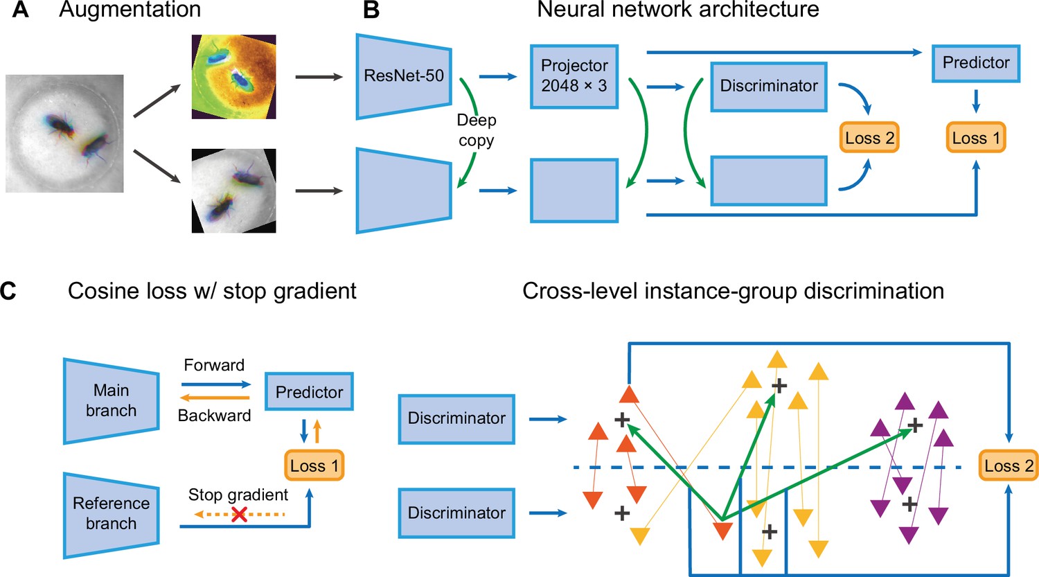
The network structure of Selfee (Self-supervised Features Extraction).
(A) The architecture of Selfee networks. Each live-frame is randomly transformed twice before being fed into Selfee. Data augmentations include crop, rotation, flip, Turbo, and color jitter. (B) Selfee adopts a SimSiam-style network structure with additional group discriminators. Loss 1 is canonical negative cosine loss, and loss 2 is the newly proposed CLD (cross-level instance-group discrimination) loss. (C) A brief illustration of two loss terms used in Selfee. The first term of loss is negative cosine loss, and the outcome from the reference branch is detached from the computational graph to prevent mode collapse. The second term of loss is the CLD loss. All data points are colored based on the clustering result of the upper branch, and points representing the same instance are attached by lines. For one instance, the orange triangle, its representation from one branch is compared with cluster centroids of another branch and yields affinities (green arrows). Loss 2 is calculated as the cross-entropy between the affinity vector and the cluster label of its counterpart (blue arrows).
Figure 2—figure supplement 1
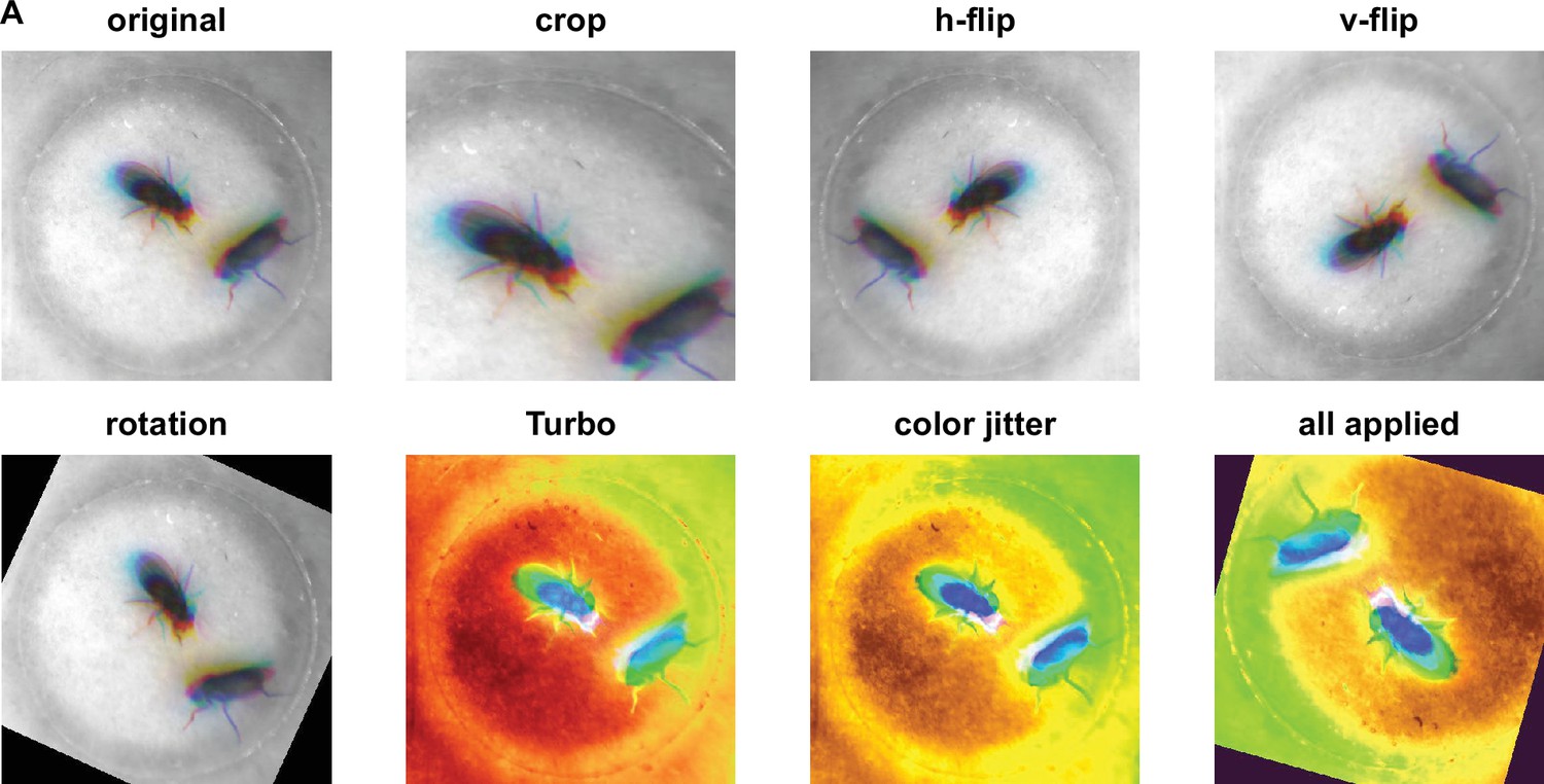
Different augmentations used for Selfee (Self-supervised Features Extraction) training.
(A) Visualization of each augmentation. For data augmentations, crop, rotation, flip, Turbo, and color jitter were applied. Each live-frame was randomly cropped into a smaller version containing more than 49% (70%×70%) of the original image; then the image was randomly (clockwise or anticlockwise) rotated for an angle smaller than the acute angle formed by the diagonal line and the vertical line, then the image would be vertically flipped, horizontally flipped, and/or applied the Turbo lookup table at the probability of 50%, respectively; and finally, the brightness, contrast, saturation, and hue were randomly adjusted within 10% variation. Detailed descriptions of each augmentation could be found in the Materials and methods and source codes.
Figure 3 with 6 supplements
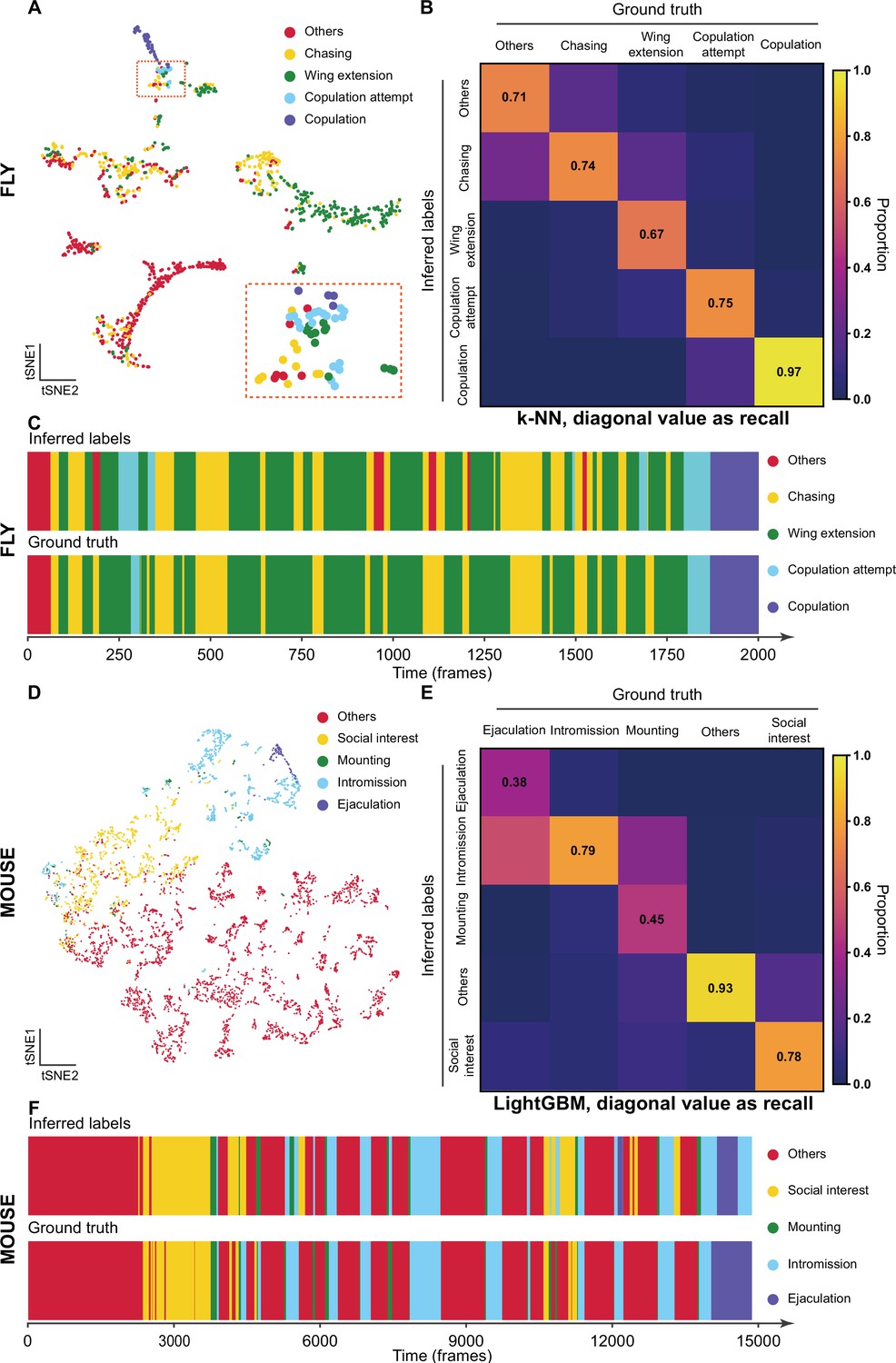
The validation of Selfee (Self-supervised Features Extraction) with human annotations.
(A) Visualization of fly courtship live-frames with t-SNE dimension reduction. Each dot was colored based on human annotations. Points representing chasing, wing extension, copulation attempt, copulation, and non-interactive behaviors (‘others’) were colored with yellow, green, blue, violet and red, respectively. (B) The confusion matrix of the k-NN classifier for fly courtship behavior, normalized by the numbers of each behavior in the ground truth. The average F1 score of the sevenfold cross-validation was 72.4%, and mAP was 75.8%. The recall of each class of behaviors was indicated on the diagonal of the confusion matrix. (C) A visualized comparison of labels produced by the k-NN classifier and human annotations of fly courtship behaviors. The k-NN classifier was constructed with data and labels of all seven videos used in the cross-validation, and the F1 score was 76.1% and mAP was 76.1%. (D) Visualization of live-frames of mice mating behaviors with t-SNE dimension reduction. Each dot is colored based on human annotations. Points representing non-interactive behaviors (‘others’), social interest, mounting, intromission, and ejaculation were colored with red, yellow, green, blue, and violet, respectively. (E) The confusion matrix of the LightGBM (Light Gradient Boosting Machine) classifier for mice mating behaviors, normalized by the numbers of each behavior in the ground truth. For the LightGBM classifier, the average F1 score of the eightfold cross-validation was 67.4%, and mAP was 69.1%. The recall of each class of behaviors was indicated on the diagonal of the confusion matrix. (F) A visualized comparison of labels produced by the LightGBM classifier and human annotations of mice mating behaviors. An ensemble of eight trained LightGBM was used, and the F1 sore was 68.1% and mAP was not available for this ensembled classifier due to the voting mechanism.
Figure 3—figure supplement 1
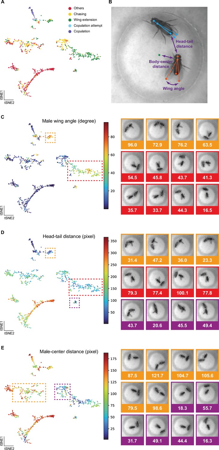
Selfee (Self-supervised Features Extraction) captured fine-grained features related to animal postures and positions.
(A) Visualization of fly courtship live-frames with t-SNE dimension reduction. Each dot was colored based on human annotations. Points representing non-interactive behaviors (‘others’), chasing, wing extension, copulation attempt, and copulation were colored with red, yellow, green, blue, and violet, respectively. Same as Figure 3A. (B) Fly skeletons were semi-automated labeled, and three features were used in the following panels. Five body parts were marked with points, including head, tail, thorax, wings, and head to tail, thorax to wings were linked by lines. Females were indicated by blue color and males were indicated by orange color. Three features were male head to female tail distance, male thorax to chamber center, and the angle between male wings, which were indicated in violet. (C) Male wing angles were visualized on the t-SNE map same as panel A. Frames of wing extension behaviors in the red box were of relatively smaller wing angles than those in the orange box. Some examples from these two groups were exhibited on the right, with their angle values below each image. (D) Male head to female tail distances were visualized on the t-SNE map same as panel A. Frames of wing extension behaviors in the red box were of relatively shorter distance than those in the orange and violet boxes. Some examples from these three groups were exhibited on the right, with their distance values below each image. (E) Male thorax to chamber center distances were visualized on the t-SNE map same as panel A. Frames of chasing behaviors in the violet box were of relatively shorter distance than those in the orange box. Some examples from these two groups were exhibited on the right, with their distance values below each image.
Figure 3—figure supplement 2
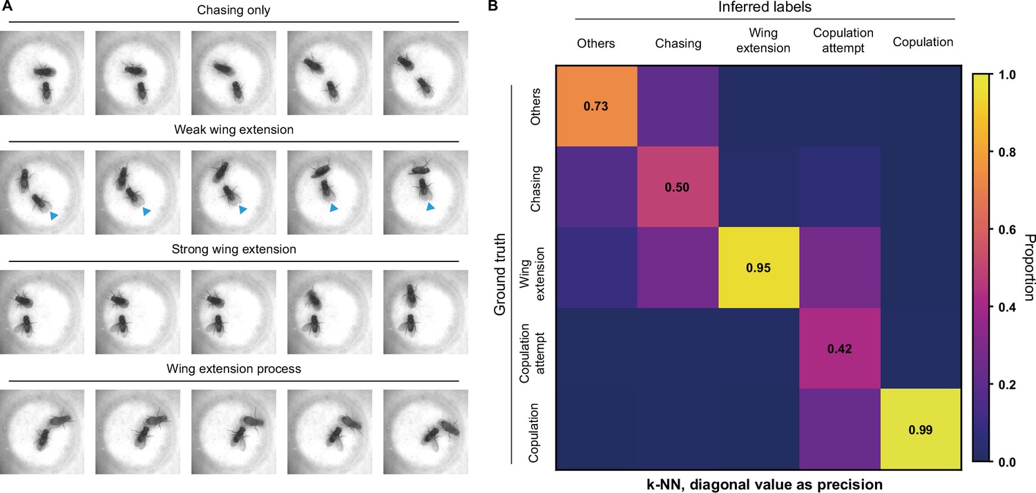
Difficulties on fly courtship behavior classification.
(A) Some wing extension frames are hard to distinguish from chasing behaviors. Images in the first row were labeled as no wing extension; images in the second to the fourth rows were labeled as wing extension. Images in the second row were of relatively weak wing extension (blue indicators pointed at slightly extended wings), and the fourth row showed a process from no wing extension to strong wing extension. (B) The confusion matrix of the k-NN classifier, normalized by the numbers of each behavior in inferred labels. The average F1 score of the sevenfold cross-validation was 72.4%, and mAP was 75.8%. The precision of each class of behaviors was indicated on the diagonal of the confusion matrix.
Figure 3—figure supplement 3
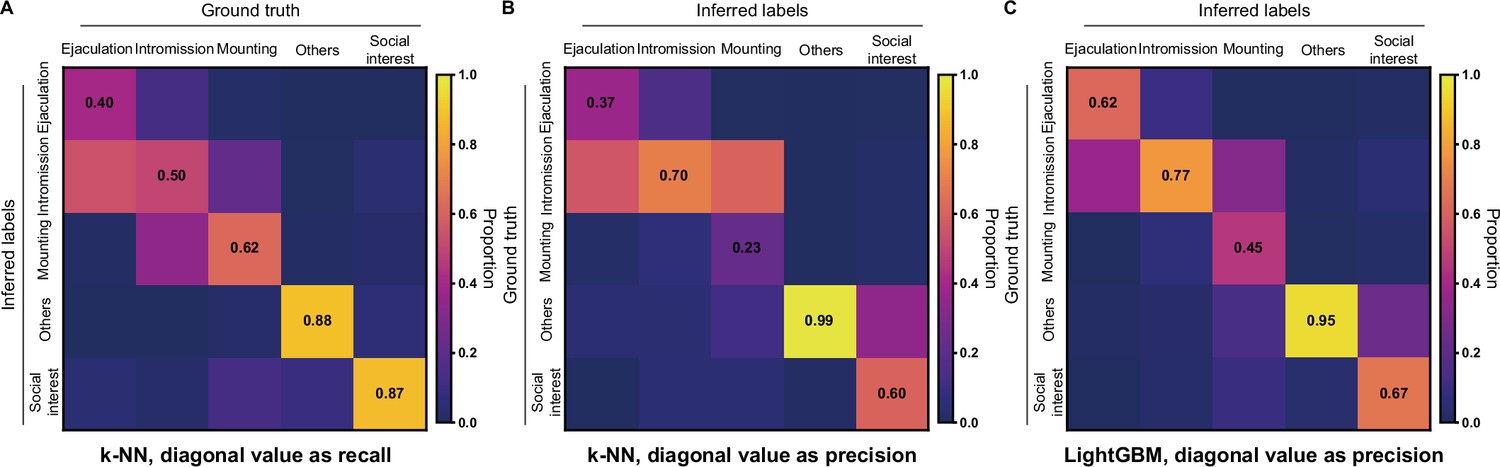
Classification of mice mating behaviors with Selfee (Self-supervised Features Extraction) extracted features.
(A) For the k-NN classifier, the average F1 score of the eightfold cross-validation was 59.0%, and mAP was 53.0%. The confusion matrix of the k-NN classifier, normalized by the numbers of each behavior in the ground truth. The recall of each class of behaviors was indicated on the diagonal of the confusion matrix. (B) The confusion matrix of the k-NN classifier, normalized by the numbers of each behavior in inferred labels. The precision of each class of behaviors was indicated on the diagonal of the confusion matrix. (C) The confusion matrix of the LightGBM (Light Gradient Boosting Machine) classifier, normalized by the numbers of each behavior in inferred labels. The precision of each class of behaviors was indicated on the diagonal of the confusion matrix. The LightGBM classifier had a much better performance compared with the k-NN classifier.
Figure 3—figure supplement 4
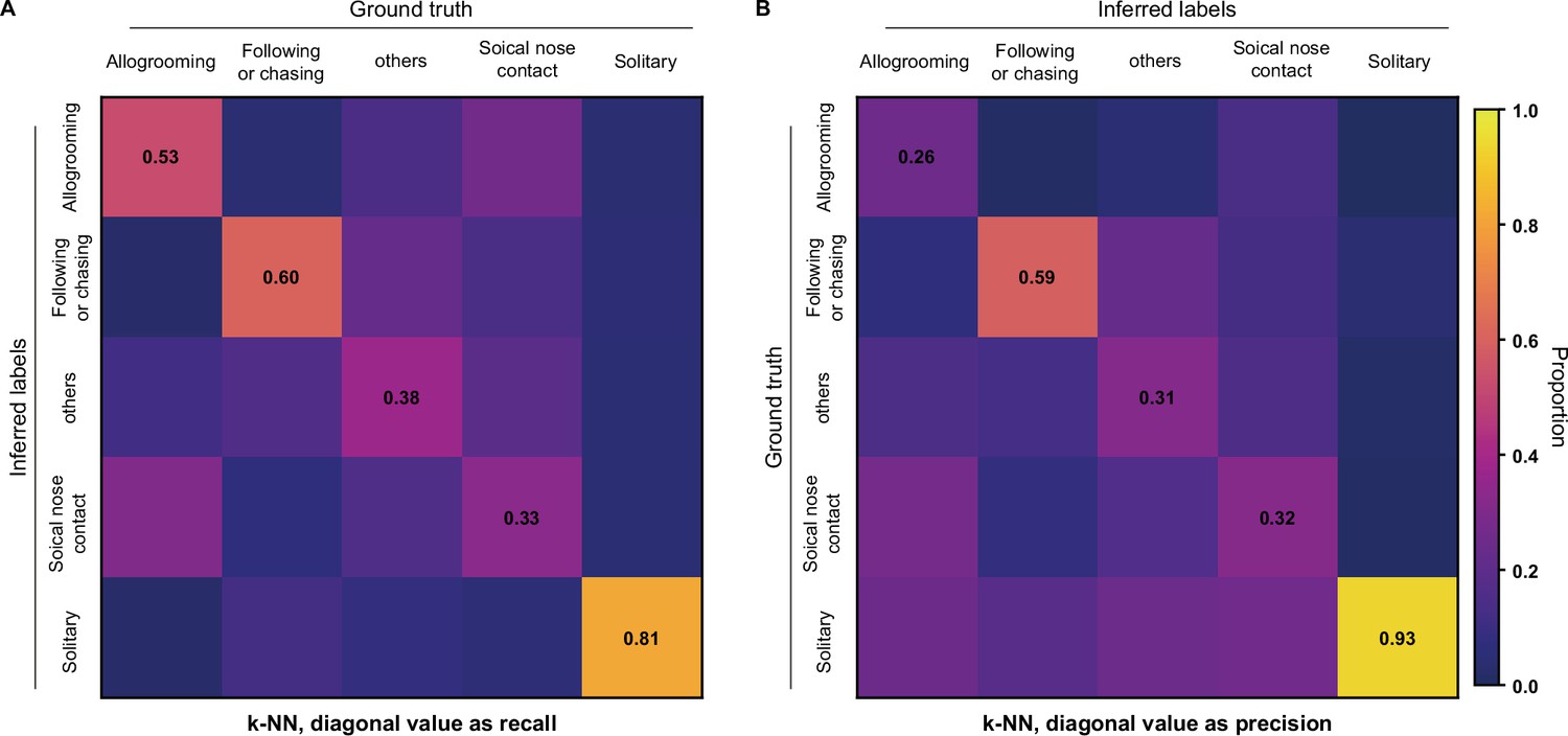
k-NN classification of rat behaviors with Selfee (Self-supervised Features Extraction) trained on mice datasets.
(A) The average F1 score of the ninefold cross-validation was 49.6%, and mAP was 46.6%. The confusion matrix of the k-NN classifier, normalized by the numbers of each behavior in the ground truth. The recall of each class of behaviors was indicated on the diagonal of the confusion matrix. (B) The confusion matrix of the k-NN classifier, normalized by the numbers of each behavior in inferred labels. The precision of each class of behaviors was indicated on the diagonal of the confusion matrix.
Figure 3—figure supplement 5
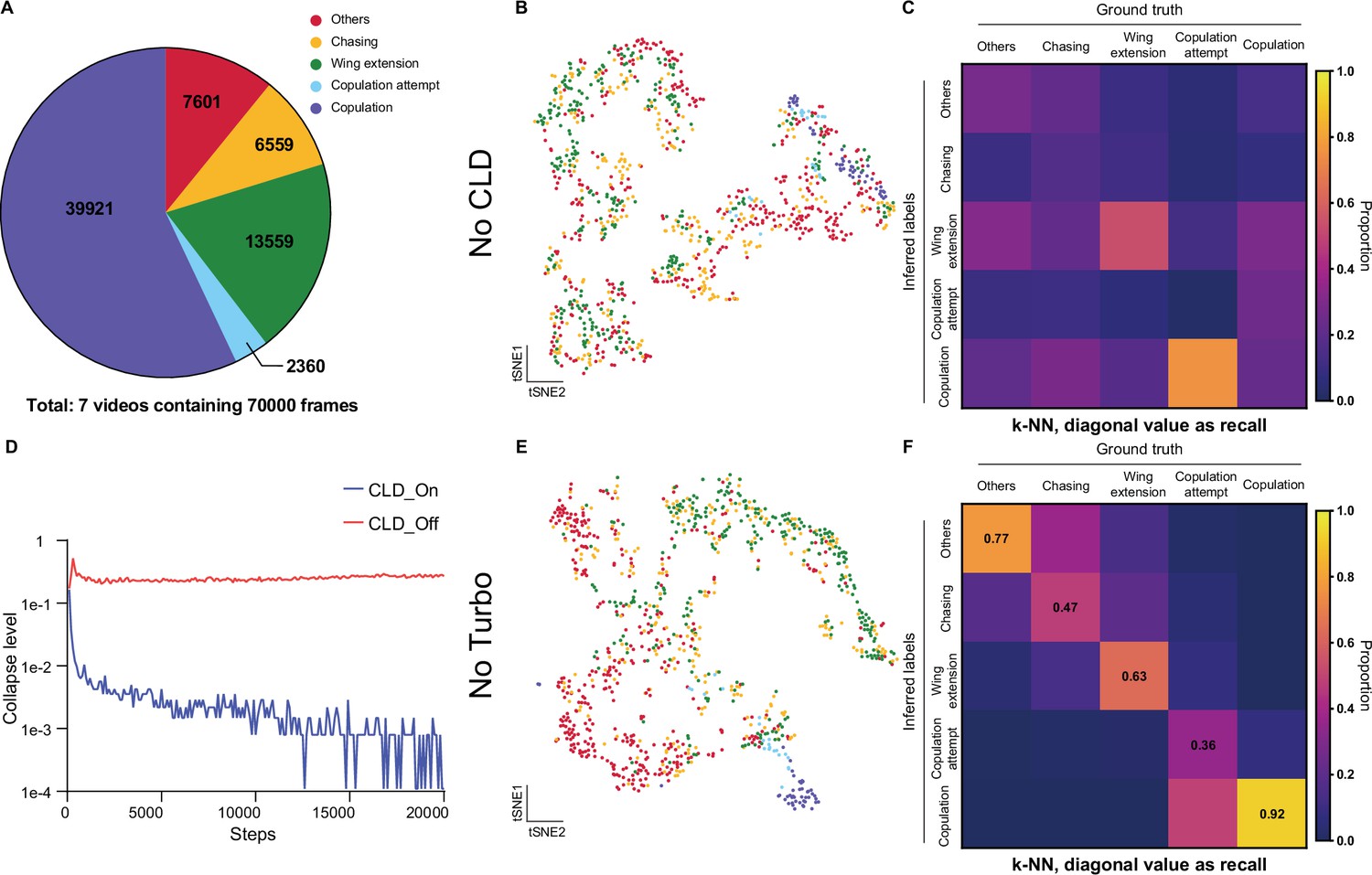
Ablation test of Selfee (Self-supervised Features Extraction) training process on fly datasets.
(A) The distribution of different behaviors in wild-type flies courtship videos. (B) Visualization of the same live-frames as Figure 3A with t-SNE dimension reduction. Used representations were extracted by models trained without cross-level instance-group discrimination (CLD) loss. Each dot is colored based on human annotations. The legend is shared with panel A. (C) The confusion matrix of the k-NN classifier, normalized by the numbers of each behavior in the ground truth. The recall of each class of behaviors was indicated on the diagonal of the confusion matrix. Used representations were extracted by models trained without CLD loss. (D) Collapse levels during the training process. Collapse level was calculated as one minus to the average standard deviation of each channel of the representation multiplied by the square root of the channel number. One means maximum collapse, while zero means no collapse. Without CLD loss, Selfee suffered from catastrophic mode collapse. Details for collapse level calculation could be found in Materials and methods. (E) Visualization of the same live-frames as Figure 3A with t-SNE dimension reduction. Used representations were extracted by models trained without Turbo transformation. Each dot is colored based on human annotations. The legend is shared with panel A. (F) The confusion matrix of the k-NN classifier, normalized by the numbers of each behavior in the ground truth. The recall of each class of behaviors was indicated on the diagonal of the confusion matrix. Used representations were extracted by models trained without Turbo transformation.
Figure 3—video 1
Pose estimation of fly courtship behaviors.
Flies’ wings, heads, tails, and thoraxes were tracked throughout the clip automatically using cutting-edge animal tracking software SLEAP, and each frame was carefully manual proofread by human researchers.
Figure 4 with 3 supplements

Anomalous posture detection using Selfee (Self-supervised Features Extraction)-produced features.
(A) The calculation process of anomaly scores. Each query frame is compared with every reference frame, and the nearest distance was named IES (the thickness of lines indicates distances). Each query frame is also compared with every query frame, and the nearest distance is called IAS. The final anomaly score of each frame equals IES minus IAS. (B) Anomaly detection results of 15 fly lines with mutations in neurotransmitter genes or with specific neurons silenced ( n = 10,9,10,7,12,15,29,7,16,8,8,6,7,7,9,7, respectively). RA is short for CCHa2-R-RA, and RB is short for CCHa2-R-RB. CCHa2-R-RBGal4>Kir2.1, q<0.0001; TrhGal4, q=0.0432; one-way ANOVA with Benjamini and Hochberg correction. (C) Examples of mixed tussles and copulation attempts identified in CCHa2-R-RBGal4>Kir2.1 flies. (D) The temporal dynamic of anomaly scores during the mixed behavior, centralized at 1.67 s. SEM is indicated with the light color region. (E) Examples of close body contact behaviors identified in TrhGal4 flies. (F) The cosine similarity between the center frame of the close body contact behaviors (1.67 s) and their local frames. SEM is indicated with the light color region. (G) The kicking index of TrhGal4 flies (n=30) was significantly lower than w1118 flies (n=27), p=0.0034, Mann-Whitney test. (H) Examples of social aggregation behaviors of TrhGal4 flies and w1118 flies. Forty male flies were transferred into a vertically placed triangle chamber (blue dashed lines), and the photo was taken after 20 min. A fly was indicated by a blue arrow. The lateral sides of the chamber were 16.72 cm. (I) Social distances of TrhGal4 flies (n=6) and w1118 flies (n=6). TrhGal4 flies had much closer social distances with each other compared with w1118 flies; nearest, p=0.0043; median, p=0.002; average, p=0.0087; all Mann-Whitney test. (J) Distributions of the median social distance of TrhGal4 flies and w1118 flies. Distributions were calculated within each replication. Average distributions were indicated with solid lines, and SEMs were indicated with light color regions.
Figure 4—figure supplement 1
Using intra-group score (IAS) to eliminate false-positive results in anomaly detections.
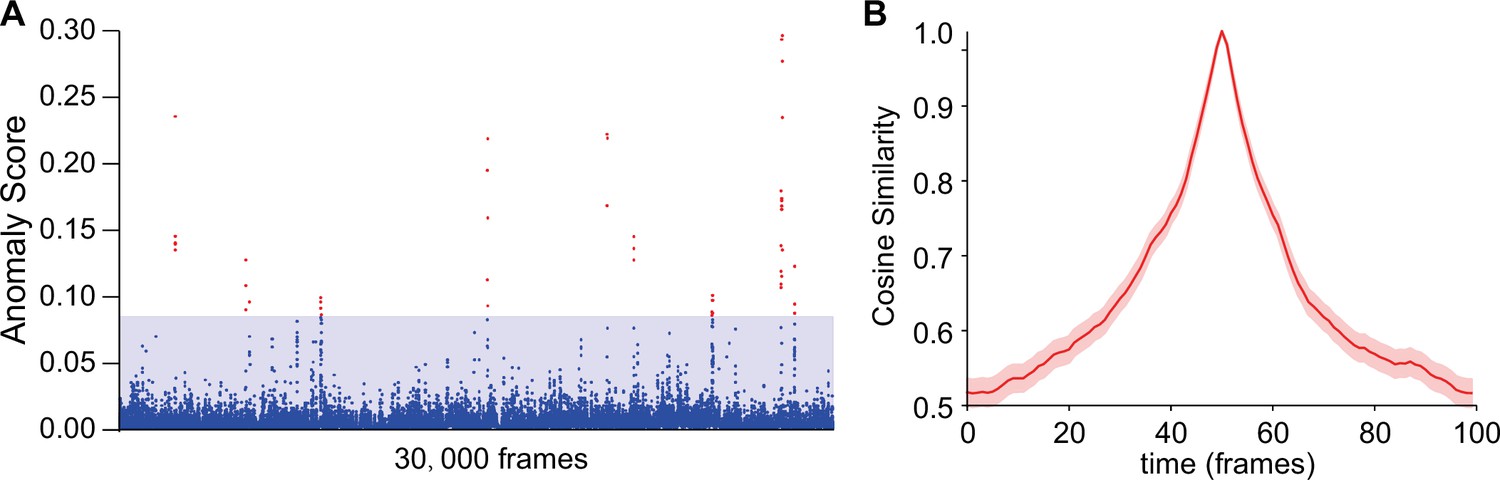
(A) Anomaly scores without IAS of wild-type male-male interactions with the same genotype as references. The blue region indicates the max anomaly score when using IAS; blue dots indicate anomaly scores without IAS that fall into the blue region; red dots indicate false-positive anomaly scores. (B) The cosine similarity between the center frame of wild-type courtship behaviors (1.67 s) and their local frames. SEM is indicated with the light color region. Seven videos containing 70,000 frames were split into non-overlapping 100-frame fragments for calculations. Beyond ±50 frames, the cosine similarity dropped to a much lower level, not affecting anomaly detection.
Figure 4—video 1
The anomaly detection on male-male interactions of RB-Gal4 >Kir2.1 flies.
The anomalous behavior was brief tussle behavior mixed with copulation attempts. This behavior was ultra-fast and lasted for less than a quarter second.
Figure 4—video 2
The anomaly detection on male-male interactions of TrhGal4 flies.
The anomalous behavior was short-range body interactions. These social interactions could last for around half to 1 s on average.
Figure 5 with 2 supplements

Time-series analyses using Selfee (Self-supervised Features Extraction)-produced features.
(A) A brief illustration of the autoregressive hidden Markov model (AR-HMM). The local autoregressive property is determined by βt, the autoregressive matrix, which is yield based on the current hidden state of the HMM. The transition between each hidden state is described by the transition matrix (pij). (B) Principal component analysis (PCA) visualization of state usages of mice in control groups (n=17, blue points) and chronic immobilization stress (CIS) groups (n=17, red points). (C) State usages of 10 modules. Module No.0 and No.3 showed significantly different usages in wild-type and mutant flies; p=0.00065, q=0.003 and p=0.015, q=0.038, respectively, Mann-Whitney test with Benjamini and Hochberg correction. (D) The differences spotted by the AR-HMM could be explained by the mice’s position. Mice distances to the two nearest walls were calculated in each frame. Distance distributions (the bin width was 1 cm) throughout open-field test (OFT) experiments were plotted in solid lines, and SEMs were indicated with light color regions. Green blocks indicated bins with statistic differences between the CIS group and control groups. Frames assigned to modules No.0 and No.3 were isolated, and their distance distributions were plotted in blue and yellow bars, respectively. Frames of module No.0 were enriched in bins of larger values, while frames of module No.3 were enriched in bins of smaller values. (E) A brief illustration of the dynamic time warping (DTW) model. The transformation from a rounded rectangle to an ellipse could contain six steps (gray reference shapes). The query transformation lags at step 2 but surpasses at step 4. The dynamic is visualized on the right panel. (F) NorpA36 flies (n=6) showed a significantly longer copulation latency than wild-type flies (n=7), p=0.0495, Mann-Whitney test. (G) NorpA36 flies had delayed courtship dynamics than wild-type flies with DTW visualization. Dynamic of wild-type flies and NorpA mutant flies were indicated by blue and red lines, respectively, and SEMs were indicated with light color regions. The red line was laid below the blue line, showing a delayed dynamic of NorpA mutant flies.
Figure 5—video 1
A video example of Module No.0.
An exploratory-like behavior of mice.
Figure 5—video 2
A video example of Module No.3.
Mice walking alongside walls of the arena.
Figure 6 with 2 supplements
Application of the Selfee (Self-supervised Features Extraction) pipeline to mice open-field test (OFT) videos.
(A) Image preprocessing for Selfee. The area of the behavior chamber was cropped, and the background was extracted. Illumination normalization was performed after background subtraction. This preprocessing could be skipped if the background was consistent in each video, as our pipeline for fly videos (dashed lines). (B) Anomaly detection of mice OFT videos after chronic immobilization stress (CIS) experiences. Only 12 frames (red points, indicated by arrows) were detected based on a threshold constructed with control mice (the blue region), and anomaly scores were slightly higher than the threshold. (C) Dynamic time warping (DTW) analysis of mice OFT videos after CIS experiences. The dynamic difference between control groups and CIS groups was visualized, and positive values indicated a delay of the reference (control groups). Results from Selfee features and animal positions were similar (red and blue lines, respectively). (D) Autoregressive hidden Markov model (AR-HMM) analysis of mice OFT videos after CIS experiences. Principal component analysis (PCA) visualization of state usages of mice in control groups (n=17, blue points) and CIS groups (n=17, red points). Same as Figure 5B.
Figure 6—figure supplement 1
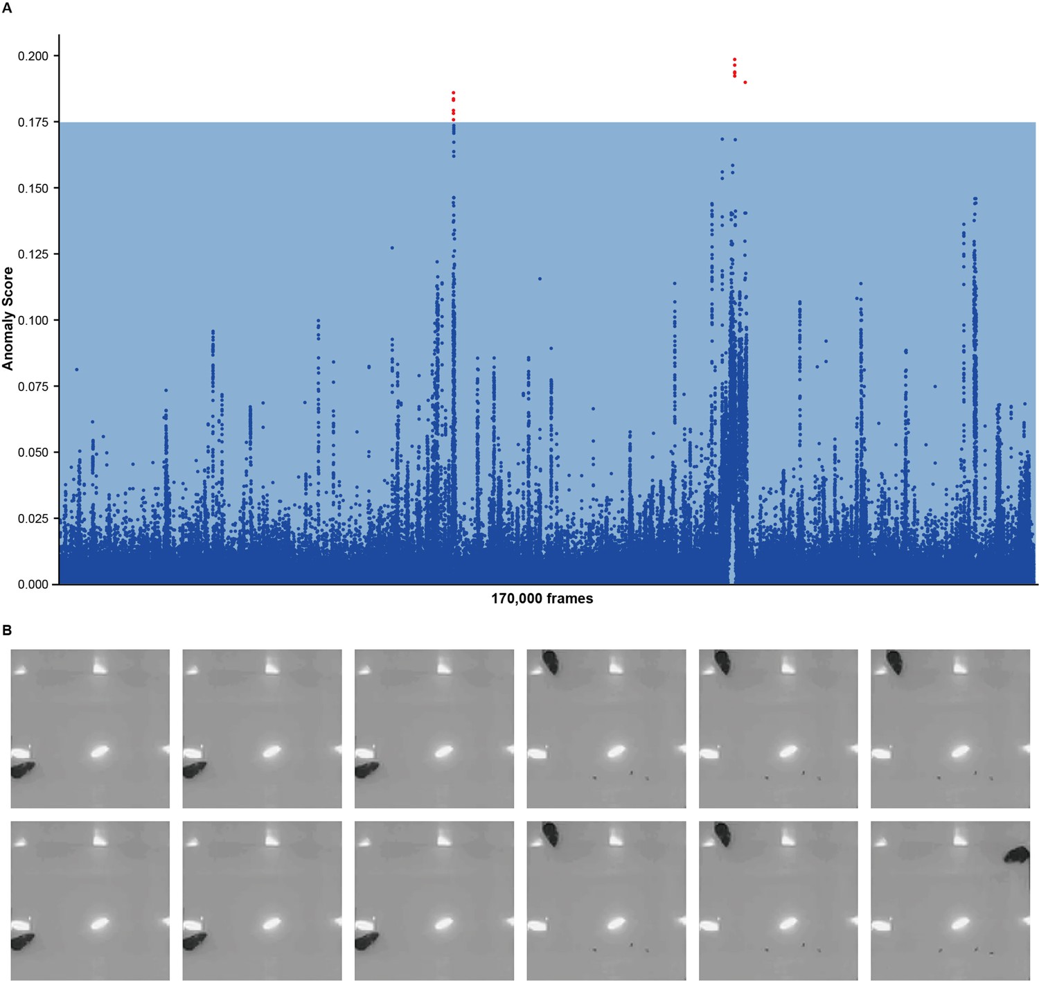
Anomaly detection of chronic immobilization stress (CIS) mice.
(A) Anomaly scores of CIS mice with half of mice in the control groups as references and another half as negative controls. The blue region indicates the max anomaly score of negative controls; blue dots indicate anomaly scores fall into the blue region; red dots indicate detected anomalies (12 points in total). Detected anomalies were only of scores slightly higher than the threshold. (B) Twelve anomalous frames. These frames contained mice near walls with their head facing the center of the arena. All frames seemed normal.
Figure 6—figure supplement 2
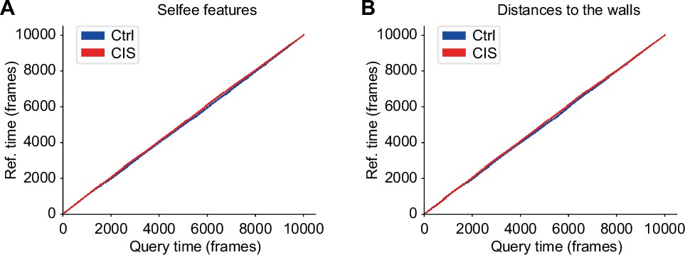
Dynamic time warping (DTW) analysis of chronic immobilization stress (CIS) and control mice.
(A) DTW analysis using Selfee (Self-supervised Features Extraction) features of mice in CIS groups with control mice as reference. The red line represents CIS groups, and the blue line represents control groups. The red line is slightly above the blue line. (B) DTW analysis using mice distances to two nearest walls of mice in CIS groups with control mice as reference. The red line represents CIS groups, and the blue line represents control groups. The red line is slightly above the blue line.
Tables
Table 1
A comparison between Selfee (Self-supervised Features Extraction) extracted features and animal-tracking derived features.
| Evaluationssetups | Pearson’s R | F1 score | AP |
|---|---|---|---|
| Selfee | 0.774* | 0.629* | 0.354 |
| FlyTracker ->FlyTracker | 0.756 | 0.571 | 0.330 |
| FlyTracker ->JAABA | 0.755 | 0.613 | 0.346 |
| FlyTracker (w/o legs) ->distance | 0.771 | 0.613 | 0.374* |
| FlyTracker (w/ legs) ->distance | 0.629 | 0.400 | 0.256 |
-
*
Best results of different feature extractors under each evaluation metric are indicated in bold values.
Table 2
An ablation test of Selfee (Self-supervised Features Extraction) training process on fly datasets.
| Model | Pre-trained ResNet-50 with random projectors | Selfee | Selfee without CLD loss | Selfee without Turbo transformation | ||||
|---|---|---|---|---|---|---|---|---|
| Evaluation | Mean F1 score | Mean AP | Mean F1 score | Mean AP | Mean F1 score | Mean AP | Mean F1 score | Mean AP |
| Replication 1 | 0.586 | 0.580 | 0.724 | 0.758 | 0.227 | 0.227 | 0.604 | 0.550 |
| Replication 2 | 0.597 | 0.570 | 0.676 | 0.683 | 0.163 | 0.200 | 0.574 | 0.551 |
| Replication 3 | 0.596 | 0.586 | 0.714 | 0.754 | 0.172 | 0.214 | 0.517 | 0.497 |
| Best | 0.597 | 0.586 | 0.724* | 0.758* | 0.227 | 0.227 | 0.604 | 0.551 |
-
*
Best results of different training setups under each evaluation metric are indicated in bold values.
Table 3
An ablation test of Selfee training process on mice datasets.
| Model | Single frame + KNN | Live-frame + KNN | Single frame + LGBM | Live-frame + LGBM | ||||
|---|---|---|---|---|---|---|---|---|
| Evaluation | Mean F1 score | Mean AP | Mean F1 score | Mean AP | Mean F1 score | Mean AP | Mean F1 score | Mean AP |
| Replication 1 | 0.554 | 0.498 | 0.590 | 0.530 | 0.645 | 0.671 | 0.674 | 0.691 |
| Replication 2 | 0.574 | 0.508 | 0.599 | 0.549 | 0.653 | 0.663 | 0.663 | 0.699 |
| Replication 3 | 0.566 | 0.514 | 0.601 | 0.539 | 0.652 | 0.692 | 0.663 | 0.700 |
| Mean | 0.565 | 0.507 | 0.597 | 0.539 | 0.650 | 0.675 | 0.667* | 0.697* |
| Best | 0.574 | 0.514 | 0.601 | 0.549 | 0.653 | 0.692 | 0.674* | 0.700* |
-
*
Best results of different training setups under each evaluation metric are indicated in bold values.
Key resources table
| Reagent type (species) or resource | Designation | Source or reference | Identifiers | Additional information |
|---|---|---|---|---|
| Genetic reagent (Drosophila melanogaster) | w1118 | – | – | Female, Figure 3A–C & Figure 5F–G; male, Figure 4G–J |
| Genetic reagent (Drosophila melanogaster) | CS | – | – | Male, Figure 3A–C, Figure 4B & Figure 5F–G |
| Genetic reagent (Drosophila. melanogaster) | CCHa1attP | BDRC | 84458 | w[*]; TI{RFP[3xP3.cUa]=TI}CCHa1[attP]; male, Figure 4B |
| Genetic reagent (Drosophila melanogaster) | CCHa1-RattP | BDRC | 84459 | w[*]; TI{RFP[3xP3.cUa]=TI}CCHa1-R[attP]; male, Figure 4B |
| Genetic reagent (Drosophila melanogaster) | CCHa2attP | BDRC | 84460 | w[*]; TI{RFP[3xP3.cUa]=TI}CCHa2[attP]; male, Figure 4B |
| Genetic reagent (Drosophila melanogaster) | CCHa2-RattP | BDRC | 84461 | w[*]; TI{RFP[3xP3.cUa]=TI}CCHa2-R[attP]; male, Figure 4B |
| Genetic reagent (Drosophila melanogaster) | CCHa2-R-RAGal4 | BDRC | 84603 | TI{2 A-GAL4}CCHa2-R[2 A-A.GAL4]; with Kir2.1, Figure 4B |
| Genetic reagent (Drosophila melanogaster) | CCHa2-R-RBGal4 | BDRC | 84604 | TI{2 A-GAL4}CCHa2-R[2A-B.GAL4]; with Kir2.1, Figure 4B |
| Genetic reagent (Drosophila melanogaster) | CNMaattP | BDRC | 84485 | w[*]; TI{RFP[3xP3.cUa]=TI}CNMa[attP]; male, Figure 4B |
| Genetic reagent (Drosophila melanogaster) | OambattP | BDRC | 84555 | w[*]; TI{RFP[3xP3.cUa]=TI}Oamb[attP]; male, Figure 4B |
| Genetic reagent (Drosophila melanogaster) | Dop2RKO | BDRC | 84720 | TI{TI}Dop2R[KO]; male, Figure 4B |
| Genetic reagent (Drosophila melanogaster) | DopEcRGal4 | BDRC | 84717 | TI{GAL4}DopEcR[KOGal4.w-]; male, Figure 4B |
| Genetic reagent (Drosophila melanogaster) | SerTattP | BDRC | 84572 | w[*]; TI{RFP[3xP3.cUa]=TI}SerT[attP]; male, Figure 4B |
| Genetic reagent (Drosophila melanogaster) | TrhGal4 | BDRC | 86146 | w[*]; TI{RFP[3xP3.cUa]=2 A-GAL4}Trh[GKO]; male, Figure 4B |
| Genetic reagent (Drosophila melanogaster) | TKattP | BDRC | 84579 | w[*]; TI{RFP[3xP3.cUa]=TI}Tk[attP]; male, Figure 4B |
| Genetic reagent (Drosophila melanogaster) | UAS-Kir2.1 | BDRC | 6595 | w[*]; P{w[+mC]=UAS-Hsap\KCNJ2.EGFP}7; with Gal4, Figure 4B |
| Genetic reagent (Drosophila melanogaster) | NorpA36 | BDRC | 9048 | w[*] norpA[P24]; male, Figure 5F–G |
| Genetic reagent (Drosophila melanogaster) | Tdc2RO54 | Pan Lab at SEU | Tdc2[RO54]; male, Figure 4B | |
| Genetic reagent (Drosophila melanogaster) | Taotie-Gal4 | Zhu Lab at IBP | w[*]; P{w[+mC]=Gr28 b.b-GAL4.4.7}10; with Kir2.1, Figure 4B | |
| Genetic reagent (Mus musculus) | C57BL/6J | – | – | Figure 3D–F & Figure 5B–D |
| Software, algorithm | python | Anaconda | – | 3.8.8 |
| Software, algorithm | numpy | Anaconda | – | 1.19.2 |
| Software, algorithm | matplotlib | Anaconda | – | 3.4.1 |
| Software, algorithm | av | conda-forge | – | 8.0.3 |
| Software, algorithm | scipy | Anaconda | – | 1.6.2 |
| Software, algorithm | cudatoolkit | conda-forge | – | 11.1.1 |
| Software, algorithm | pytorch | pytorch | – | 1.8.1 |
| Software, algorithm | torchvision | pytorch | – | 0.9.1 |
| Software, algorithm | pillow | Anaconda | – | 8.2.0 |
| Software, algorithm | scikit-learn | Anaconda | – | 0.24.2 |
| Software, algorithm | pandas | Anaconda | – | 1.2.4 |
| Software, algorithm | lightgbm | conda-forge | – | 3.2.1 |
| Software, algorithm | opencv-python | PyPI | – | 4.5.3.56 |
| Software, algorithm | psutil | PyPI | – | 5.8.0 |
| Software, algorithm | pytorch-metric-learning | PyPI | – | 0.9.99 |
| Software, algorithm | pyhsmm | PyPI | – | 0.1.6 |
| Software, algorithm | autoregressive | PyPI | – | 0.1.2 |
| Software, algorithm | dtw-python | PyPI | – | 1.1.10 |
| Software, algorithm | SLEAP | conda-forge | – | 1.2.2 |
| Software, algorithm | DEEPLABCUT | PyPI | – | 2.2.0.2 |
Additional files
Download links
A two-part list of links to download the article, or parts of the article, in various formats.
Downloads (link to download the article as PDF)
Open citations (links to open the citations from this article in various online reference manager services)
Cite this article (links to download the citations from this article in formats compatible with various reference manager tools)
Selfee, self-supervised features extraction of animal behaviors
eLife 11:e76218.
https://doi.org/10.7554/eLife.76218


